
Chapter 33: Forest Inventory – Download PDF
Author: Hubert Hasenauer
Intended learning level: Basic (BSc)
This material is published under Creative Commons license CC BY-NC-SA 4.0.
| Purpose of the chapter: |
|---|
| This chapter traces the evolution of forest inventory,from early surveys and yield tables to modern systems. It clarifies inventory objectives, typical sources of bias and uncertainty, and operational constraints. Core field designs are reviewed, focusing on fixed-area plots and angle count sampling and a comparison of the two, with practical guidance on when each excels and where they fail. The chapter closes with emerging approaches that fuse terrestrial measurements with remote sensing and LiDAR. |
NOTE: this part is a full draft, which in due time will be further revised
and edited following review by the EUROSILVICS Project Board
Table of Contents
33.3.1 Stand and site elements 4
33.3.2 Variables and estimations 4
33.3.3 Static versus dynamic information 4
33.4 Inventory methods and their historic development 5
33.4.3 Sampling and Statistical Principles 5
33.5 Methods of Plot Selection 5
33.5.1 Simple Random Sampling 5
33.5.3 Stratified Systematic Sampling 6
33.5.7 Concentric (Nested) Plots 9
33.5.8 Temporary versus Permanent Sample Plots 9
33.5.9 Sampling Probability and Management Implications 11
33.6 Summary and conclusion 12
The implementation of sustainable forest management is closely linked to the development of forest inventory and growth projection methods. As early as the 18th and 19th centuries, the necessity of aligning timber use with the forest’s sustainable productive capacity was recognized (Speidel, 1972; Pretzsch, 2009). Forest data recording was needed and yield tables were developed, which allow for the prediction of future development in single-species, even-aged stands. Based on site conditions, they provide estimates of stand growth and stocking development. Site quality is described by the site index, which is derived from the mean dominant height in relation to stand age (Assmann, 1961).
For each tree species and site index, a reference stand is defined, enabling the classification of real stands by comparing their dominant tree height and age to this reference. In Austria, this concept has been further developed into a so-called Ertragsklasse (Schober, 1975), or DGZ (average total increment) site system which defines the average total increment per hectare and year for a rotation period of 100 years. This allows a more practical use of the site index system since a dgz8 for a given tree species refers to a volume growth of 8 m³/ha/year with a total volume production in 100 years of 800 m³/ha (Marschall 1975).
Although yield tables operate at the stand level and are primarily designed for even-aged pure stands, they can also be applied to mixed stands by dividing them into hypothetical pure stands. However, this approach neglects the competition dynamics both between and within tree species. To compensate, yield table values must be weighted according to the basal area of the respective species (Pretzsch, 2009).
The transition from a stand level based growth projection system as implemented in yield tables to tree growth models, is a fundamental change in ensuring sustainable forest management because no pre-defined limits in species mixture, silvicultural treatment and/or tree age exists. Tree growth models are considered a potential alternative because conceptually they predict the development of each tree within a forest. The level of resolution is the tree with its specific competition situation and this allows the required flexibility in forecasting tree growth regardless of species mixture, age distribution or applicable silvicultural system.
Historically speaking, the first tree growth models were developed in North America (see Newnham 1964, Stage 1973, Monserud 1975, Wykoff et al. 1982, Burkhart et al. 1987, Van Deusen and Biging 1985, Wensel and Koehler 1985). For Scandinavia and Central Europe, the main tree growth modeling concepts were developed during the early 90s. (For details see Sterba (1983), Pukkala (1988, 1989), Pretzsch (1992, 2001), Hasenauer (1994, 2000), Kahn and Pretzsch (1997), Pretzsch et al. (2002) Nagel (1995), Sterba et al. (1995), Monserud and Sterba (1996), Nagel et al. (2002)) These models basically extended the previous model approaches to all major species in Europe. For further details we refer to Hasenauer (19xx) or Pretzsch (2001).
33.2 The Goal of Forest Inventory
The purpose of forest inventories is to provide an accurate estimate of the current state of a forest—essentially answering the question: How much forest is there? While the specific methods of data collection have evolved, this objective has remained constant. What has changed are the motivations, which historically ranged from maximizing economic returns to implementing sustainable harvesting practices or promoting conservation (Kangas and Maltamo, 2006). Forest inventories measure not only economically relevant variables—such as volume per hectare, tree density, and growth rates—but also site conditions (e.g., soil type, damage), rare events, and past or ongoing management practices (Corona, 2016).
In the long term, inventories provide the baseline data necessary to monitor changes, support comparisons, and guide forest management decisions. Properly conducted, they represent the only standardized method for building reliable forest databases and serve as a powerful tool for both present assessments and future planning (Tomppo et al., 2010). Because standards differ widely between countries, strict adherence to national or regional protocols is essential.
Forest inventories, while essential for ensuing sustainable forest management, are subject to limitations that must be considered when interpreting results. Issues can arise from stand and site characteristics, the selection of variables, and the distinction between static (e.g. volume) and dynamic information (e.g. volume increment, which requires repeated observations or growth models).
33.3.1 Stand and site elements
Stand age, site quality, and composition strongly affect inventory outcomes. Younger stands typically exhibit faster relative growth compared to older stands, while well-managed stands on favorable sites (e.g., fully stocked versus thinned) are generally more productive. Mixed stands often resemble natural forest conditions more closely and may achieve higher growth than pure stands (Pretzsch, 2009; Bravo-Oviedo et al., 2014).
Juvenile trees are considered regeneration or understory if they fall below specific thresholds (≤ 1.3 m height or ≤ 6 cm DBH, depending on national standards). Inventories should therefore include understory data alongside site conditions. Commonly, four distinct understory height classes are recognized: ≤ 20 cm, 21–50 cm, 51–100 cm, and 101–130 cm. In addition, edge effects are estimated for trees within 60 m of stand boundaries in eight directions (Kleinn, 2000).
33.3.2 Variables and estimations
Because measuring every tree and variable is impossible, inventories rely on sampling and estimation procedures. For example, tree volume is derived from DBH, height, and a (species-specific) form factor, since trees are not perfect geometric solids (Husch et al., 2003; Avery & Burkhart, 2015). DBH is typically measured for each tree at breast height, while height is measured only for a subset of trees and then estimated for the remaining trees using allometric equations.
Stand composition also influences measurement accuracy. Young stands contain many small stems per plot, which increases random variation and reduces accuracy. In such cases, combining sampling methods can improve reliability. Older stands with greater volume per hectare generally show less variation, and most sampling techniques perform well under these conditions (Tomppo et al., 2010).
33.3.3 Static versus dynamic information
Static information refers to one-time measurements, while dynamic information involves repeated assessments over time. The latter allows for monitoring of growth and change. However, inventories often resample different trees in subsequent measurements. As long as both samples represent the population adequately, comparisons remain valid, although a degree of inaccuracy must always be accepted (Kangas and Maltamo, 2006; Corona, 2016).
33.4 Inventory methods and their historic development
There are several proven methods of selecting plots to be measured (see examples below). Each method has advantages and disadvantages, and this needs to be considered alongside the given situation and desired results.
Without systematic inventories, it is impossible to estimate (changes in) timber volume, species diversity, or age-class distribution. Historically, the lack of information about the forest situation and its development over time (= forest growth) resulted in severe overutilizing and -harvesting. Small-scale owners typically under-harvest forests since they don’t practise regular management and often are unaware of the volume of standing timber on their property, while large-scale owners historically tended to over-harvest the forests (Speidel, 1972). The first documented estimates of tree volumes appeared in the 17th century. They were based on simple approaches, such as measuring a few selected trees (e.g., the thickest or most valuable species) and extrapolating results to the whole forest (Loetsch and Haller, 1973).
Surveying or Taxation (from the Latin taxus, “estimation”) was developed for the concept of the “normal forest model.” It relied on ocular stand assessments, comparing current and projected conditions. While useful for planning, the method lacked accuracy and did not allow statistical error estimation (Kangas & Maltamo, 2006).
33.4.3 Sampling and Statistical Principles
Since it is impossible to measure every tree in a population, statistical sampling is applied.The introduction of statistical sampling was a major advance: Systematic grid-based sampling allows estimates of forest attributes from small plots, with quantifiable errors. Today, this is the most widely applied and scientifically robust method (Tomppo et al., 2010). Estimates are not true population values, but approximations with defined levels of error (Avery and Burkhart, 2015).
33.5 Methods of Plot Selection
Plot selection is a crucial step in forest inventory design. Multiple sampling methods exist, each associated with specific strengths and weaknesses. The choice of method depends on the research objective, forest conditions, and logistical considerations (Loetsch et al., 1973; Kangas & Maltamo, 2006).
In simple random sampling, every potential plot within the study area has the same probability of being selected. Plot locations are often generated using computerized random numbers. This design is statistically rigorous and unbiased, but in practice may lead to clustering of plots, leaving parts of the forest unsampled, and can require extensive travel effort (Gregoire & Valentine, 2007; West, 2016).
Systematic sampling begins with a randomly selected starting point, after which plots are laid out at regular intervals. This ensures even coverage of the study area and facilitates relocation of plots in the field. However, systematic designs may suffer from hidden periodic correlations between the grid and forest structure, potentially reducing statistical validity (Kleinn, 2007; Mandallaz, 2008).
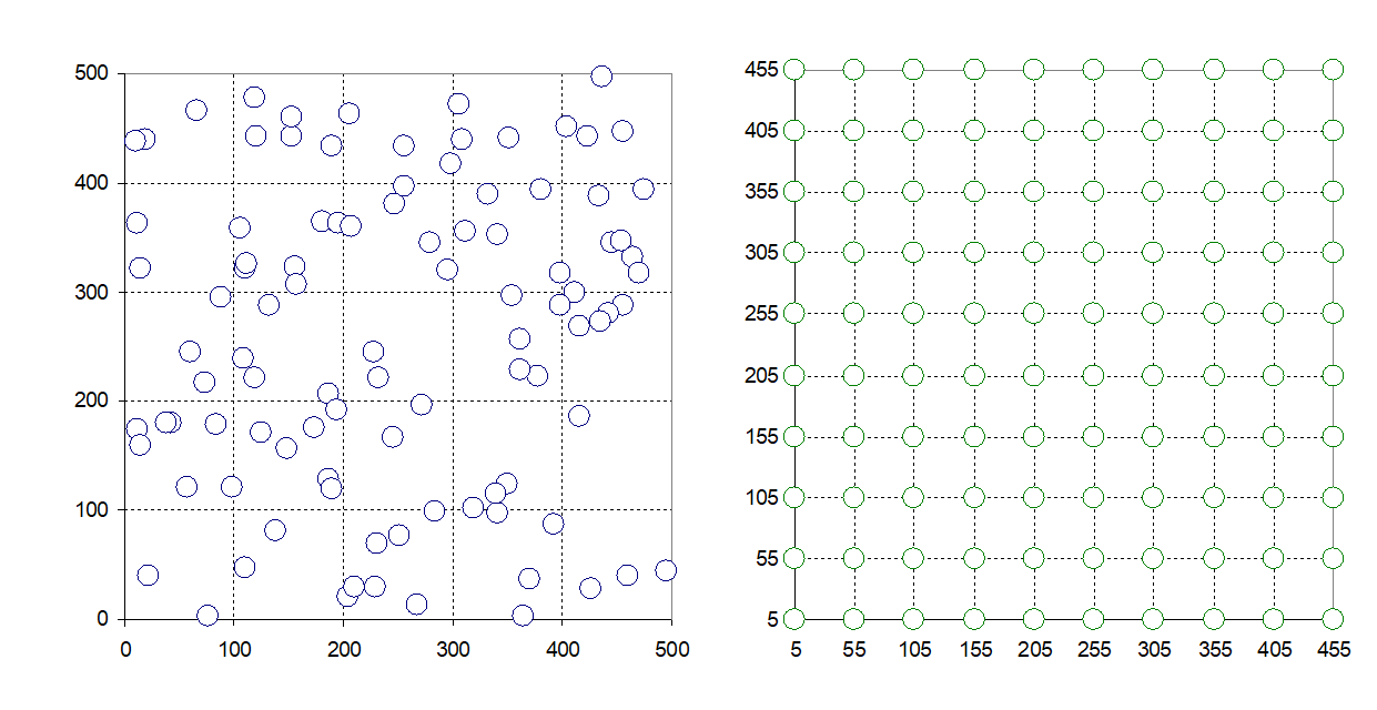
Figure 33-1: Schematic of (i) random plot selection (left) and (ii) systematic plot sampling (right)
33.5.3 Stratified Systematic Sampling
When auxiliary information about forest structure is available, the area can be divided into strata (e.g., by age class, site quality, or forest type). Within each stratum, plots are randomly or systematically selected. This approach increases precision by reducing within-stratum variability and ensuring representation across all subpopulations (Särndal et al., 1992; Corona, 2016). Its accuracy, however, depends on the quality of stratification.
Cluster sampling groups multiple plots into clusters that are then selected randomly. All plots in a cluster (single-stage) or only a subset (two-stage) may be measured. This method reduces field effort and is particularly efficient in large or remote forests, but intracluster correlation can reduce statistical efficiency (Avery & Burkhart, 2015; Rao & Wu, 2001).
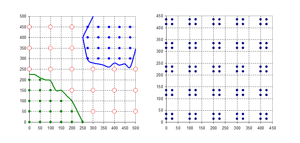
Figure 33-2: Example for (i) systematic stratified plot sampling selection (left) and (ii) systematic clustered (right) plot sampling
Fixed area plots are circular or rectangular plots in which all trees are measured. Each tree has the same probability of being sampled, making the method suitable for estimating stand density. Results are scaled to per-hectare values using a Blow-Up Factor (BF), where:

On sloping terrain, plot dimensions must be corrected for horizontal projection, since inclined surfaces distort circular plots into ellipses (Husch et al., 2003; Schreuder et al., 1993).
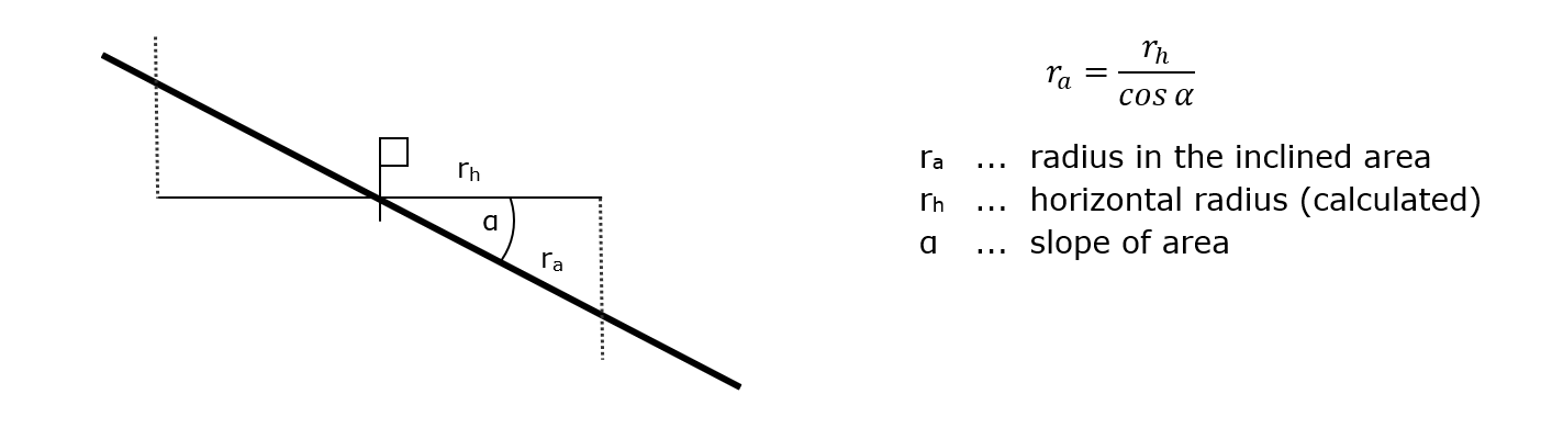
Figure 33-3: The defined fixed area plot radius is projected in inclined areas. The plot center is marked by the white flag.
Angle count sampling (ACS), introduced by Bitterlich (1948), is a probability proportional-to-size method. Tree inclusion depends on DBH and distance from the plot center, determined with a prism or angle gauge. A predetermined Basal Area Factor (BAF) allows conversion of the tally into basal area or volume per hectare. ACS is highly efficient for estimating stand volume but less reliable for estimating stem density (Kleinn, 2000; Kitikidou et al., 2011).
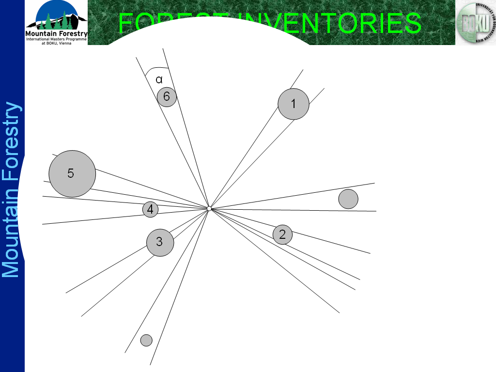
Figure 33-4: In angle count sampling, all trees that are thicker than the angle α are “in” trees and will be counted, all others are not and do not count.
Steps for Angle Count Sampling
- Mark the plot center:
- Place a stick in the ground to mark the center of the angle count sampling plot.
- Select trees to be measured
- Make a full 360° rotation around the plot center.
- For each tree, compare the width of its stem to the width of the angle count plate (Figure 4).
- If the tree stem is larger than the plate → the tree is “in”.
- If the tree stem is smaller than the plate → the tree is “out”.
- If the tree stem is the same size as the plate → the tree is “borderline”.
- Borderline tree check
- Measure the borderline radius to decide whether or not to count these trees.
- A tree is considered “in” if the measured radius (R) is less than the right-hand side of the equation:
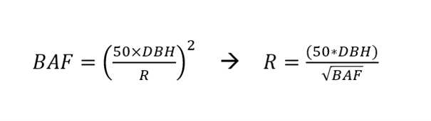
At the end of the count, the number of borderline trees is halved.
33.5.7 Concentric (Nested) Plots
Concentric plots, or nested designs, consist of multiple subplots with different radii applied to different DBH classes. Smaller trees are measured in smaller subplots, while larger trees are assessed in larger ones. This reduces fieldwork effort and provides representative data across size classes (Ståhl et al., 2016; McRoberts et al., 2018).
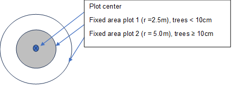
Figure 33-5: Example for a concentric circle plot, with two radii and different DBH level as thresholds.
33.5.8 Temporary versus Permanent Sample Plots
Sample plots are either temporary or permanent, depending on the aims of the forest inventory. Temporary sample plots are used to survey actual conditions, whereas permanent sample plots are used for time series of surveys. The plot center and trees must be clearly identifiable for the inventory staff. These plots should not be treated differently from the rest of the stand. One way to demarcate these plots without making them too obvious is to bury iron bars at the plot center and record the distance and angle of the trees from the plot center.
The results from two temporary plots can be compared using a t-test for independent means. The example below (Table 33-1) shows the differences in calculating the change from the 1st (T1) to the 2nd (T2) observation using either a temporary or a permanent sample plot design, and illustrates the importance of the signal-to-noise ratio.
In the temporary plot, the change in mean is less than the standard error, or in other words, the signal (mean) is weaker than the noise (standard error). This implies that we cannot make reliable statements about the development of the situation. In contrast, in the permanent plot, the mean is greater than the standard error, i.e. the signal is stronger than the noise, and thus more information regarding changes in plot measurements can be obtained.
Despite this, it should be noted that both temporary and permanent sample plot designs have advantages and disadvantages, and the most appropriate method should be chosen depending on the situation. One advantage of permanent plots is the nature of changes observed: since the same trees are measured again at T2, any changes in measurements represent true changes in those trees. With temporary plots, however, changes may simply reflect spatial variation. Temporary plots are preferable when the goal is to obtain a snapshot of the current state of the forest rather than its dynamics over time. Furthermore, they tend to be easier in terms of fieldwork (i.e. no time is required to find plots and trees again), which makes it possible to measure a larger number of plots. In summary, the choice of method ultimately depends on available financial and other resources, plot accessibility, and forest stand characteristics.
Re-measurement intervals also play an important role in the accuracy of the information obtained. In general, the signal-to-noise ratio improves with the length of the inter-measurement interval.
Table 33-1: Comparison of temporary and permanent sample plots
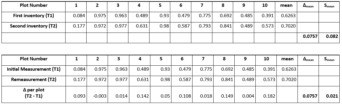
In temporary inventories, different trees are sampled at each time so changes are tested between independent samples,yielding a standard error larger than the mean (SE ≈ 0.082 > 0.0757) due to added spatial variability, whereas in permanent inventories, the same trees are remeasured and changes are paired within trees, shrinking variance via positive covariance and producing a much smaller SE (≈ 0.021 < 0.0757)
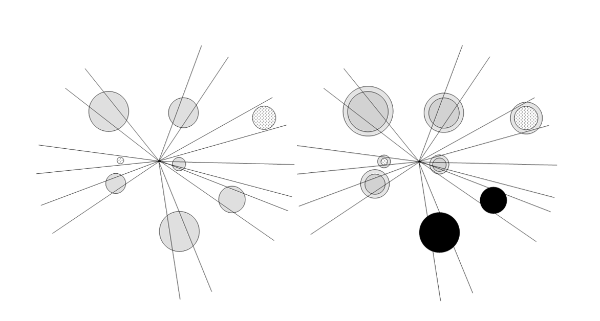
Figure 33-6: Comparison between a permanent sample plot at T1 (left) and T2 (right). At T1, the shaded trees are not part of the angle count sample, as they have no reached the required diameters. At T2, they have exceeded the borderline diameter and are now included. The trees in black have been either removed from the stand or are dead.
A temporary sample plot should be selected for its representativeness of the forest area under study. A permanent sample plot is fixed to a specific location; consequently, repeated measurements must account for mortality, harvesting, and ingrowth. Figure 33-6 compares two measurement times for a permanent plot, illustrating trees that newly meet the angle-count inclusion threshold as well as trees lost to harvest or competition-induced mortality.
Table 33-2: Advantages and Disadvantages of different sampling methods
33.5.9 Sampling Probability and Management Implications
The chosen sampling method determines the probability of tree inclusion and thus influences which parameters are estimated most precisely. Fixed area plots are more appropriate for estimating stand density, while ACS provides precise estimates of volume. In even-aged forests, volume per hectare is often prioritized, whereas in uneven-aged management, stand structure and increment across DBH classes are more relevant (Leiter & Hasenauer, 2023; Pretzsch, 2009).
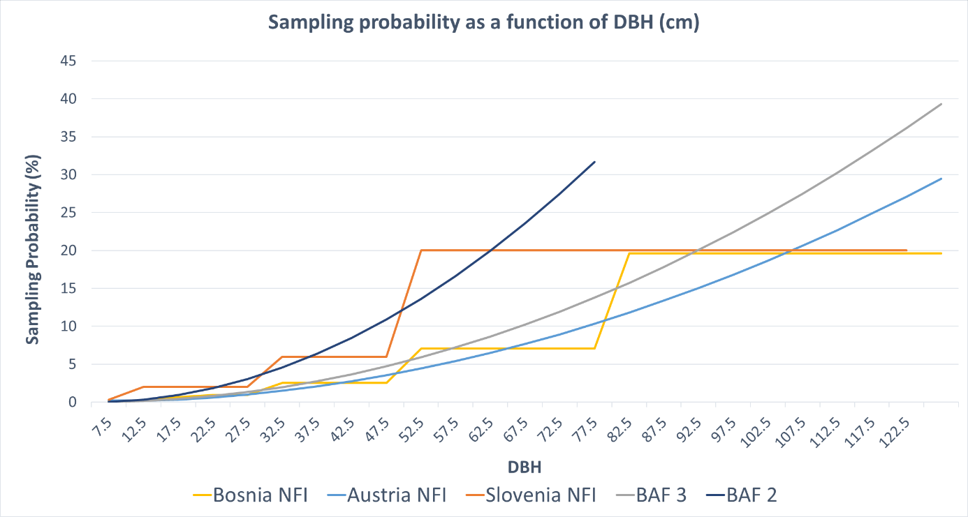
Figure 33-7: Comparison of likelihood of inclusion for different sampling methods (unpublished data).
Forest inventory ensure sustainable forest management and are defined as the systematic acquisition, analysis, and presentation of data on forest resources. Its primary objective is to provide scientifically reliable information on the quantity, quality, spatial distribution, and condition of trees and associated stand characteristics. Such information constitutes the basis for sustainable forest management, policy development, and ecological research.
Traditionally, forest inventory has relied on field-based sampling approaches. The most common designs include temporary sample plots, which provide a snapshot of the current state of the forest, and permanent sample plots, which enable the monitoring of long-term structural and compositional changes. Core measurements include tree species, diameter at breast height (DBH), tree height, volume, and site-related variables. Methods such as fixed-area plots and angle count sampling remain central to these surveys. The validity of the inventory results is determined by the sampling design, the intensity of data collection, and the frequency of re-measurements.
Recent years have witnessed a profound transformation of forest inventory practices through the integration of emerging technologies. Remote sensing techniques, in particular LiDAR (Light Detection and Ranging) and high-resolution satellite imagery, allow for large-scale and spatially explicit assessment of forest structure and biomass. Unmanned aerial vehicles (UAVs) provide flexible and high-resolution data acquisition, especially in remote or inaccessible areas. Geographic Information Systems (GIS) enable the integration and spatial analysis of diverse data sources. In addition, methods from machine learning and artificial intelligence are increasingly employed for automated tree detection, species classification, and growth modelling.
Looking ahead, the combination of traditional field measurements with advanced remote sensing and digital technologies is expected to result in more efficient, accurate, and cost-effective forest inventories. Future developments will likely focus on near-real-time monitoring systems, improved carbon accounting in the context of climate change mitigation, and comprehensive assessments of forest ecosystem services beyond timber production.
Avery, T. E., & Burkhart, H. E. (2015). Forest measurements (6th ed.). Waveland Press.
Bitterlich, W. (1948). Die Winkelzählprobe. Allgemeine Forst- und Holzwirtschaftliche Zeitung, 59, 4–5.
Corona, P. (2016). Consolidating new paradigms in large-scale monitoring and assessment of forest ecosystems. Environmental Research, 144, 8–14. https://doi.org/10.1016/j.envres.2015.11.006
Gregoire, T. G., & Valentine, H. T. (2007). Sampling strategies for natural resources and the environment. Chapman & Hall/CRC.
Husch, B., Beers, T. W., & Kershaw, J. A. (2003). Forest mensuration (4th ed.). Wiley.
Kangas, A., & Maltamo, M. (2006). Forest inventory: Methodology and applications. Springer. https://doi.org/10.1007/1-4020-4381-3
Kitikidou, K., Milios, E., Pipinis, E., & Stampoulidis, A. (2011). Comparison of angle count and fixed area sampling methods in uneven-aged stands. Annals of Forest Research, 54(1), 61–70.
Kleinn, C. (2000). On large-area inventory and assessment of trees outside forests. Unasylva, 51(200), 3–10.
Kleinn, C. (2007). A critical review of design options for forest inventories. EFI Proceedings, 57, 9–18.
Leiter, T., & Hasenauer, H. (2023). Sampling strategies for uneven-aged forest management. Forest Ecosystems, 10(1), 12. https://doi.org/10.1186/s40663-023-00456-9
Loetsch, F., Zöhrer, F., & Haller, K. E. (1973). Forest inventory (Vols. 1–2). BLV Verlagsgesellschaft.
Mandallaz, D. (2008). Sampling techniques for forest inventories. Chapman & Hall/CRC.
McRoberts, R. E., Chen, Q., Domke, G. M., Ståhl, G., Saarela, S., Westfall, J. A., & Walters, B. F. (2018). Using a remote sensing–based, percent tree cover map to enhance forest inventory estimation. Forest Ecology and Management, 430, 467–476. https://doi.org/10.1016/j.foreco.2018.08.048
Pretzsch, H. (2009). Forest dynamics, growth and yield. Springer.
Rao, J. N. K., & Wu, C. F. J. (2001). Bootstrap methods for complex surveys. Statistical Methods in Medical Research, 10(4), 283–303.
Särndal, C.-E., Swensson, B., & Wretman, J. (1992). Model assisted survey sampling. Springer.
Schreuder, H. T., Gregoire, T. G., & Wood, G. B. (1993). Sampling methods for multiresource forest inventory. Wiley.
Ståhl, G., Holm, S., Gregoire, T. G., Gobakken, T., Næsset, E., & Nelson, R. (2016). Model-based inference for biomass estimation in a LiDAR sample survey in Hedmark County, Norway. Canadian Journal of Forest Research, 46(6), 716–725. https://doi.org/10.1139/cjfr-2015-0361
West, P. W. (2016). Tree and forest measurement (3rd ed.). Springer.
33.8 Acknowledgements
This Chapter is published on the EUROSILVICS platform, established as part of the EUROSILVICS Erasmus+ grant agreement No. 2022-1-NL01-KA220-HED-000086765.
This chapter is based on the course materials of Univ.-Prof. Dr. DDr. hc. Hubert Hasenauer for the course “Forest Inventory” formerly taught by him at the University of Natural Resources and Life Sciences in Vienna, Austria. The text has been revised and updated for the EUROSILVICS project.
Author affiliation:
| Hubert Hasenauer | University of Natural Resources and Life Sciences Vienna, Austria |