Chapter 19: Radiation, energy balance and microclimate – Download PDF
Authors: Frits Mohren, Marco Nathkin, Peter Spathelf, Ute Sass-Klaassen
Author affiliations are given at the end of the chapter
Intended learning level: Basic
This material is published under Creative Commons license CC BY-NC-SA 4.0.
| Purpose of the chapter: |
|---|
| This chapter aims to introduce the main elements that determine the forest microclimate, and provides the functional link between forest canopy structure and microclimate, with solar radiation as the main driving factor. |
NOTE: this text is a complete draft, which will be further revised
and edited following review by the EUROSILVICS Project Board
19.3 Radiation behaviour in vegetation 3
19.3.1 Reflection and transmission 3
19.5 Efficiency in radiation conversion 10
19.6.1 Energy balance components 11
19.6.2 Energy balance dynamics 12
19.8 Synthesis: Effects of trees and forests on microclimate 17
This chapter deals with radiation and light interception in forests, and the energy balance determined by radiation interception by the forest canopy. Solar radiation is the main driver for meteorological variables such as temperature and the relationship between forest structure and solar radiation via light interception; and light transmission determines the energy balance of the vegetation. As a result of forest structure, this leads to significant differences between the microclimate inside a forest and the conditions in the open land. Some attention is also paid to the microclimate in a forest, and how this is determined by the forest structure in combination with the radiation, energy balance and water balance (see Chapter 20). Light interception by leaves and needles underlies photosynthesis and thus the growth of trees and forests. Quantification of radiative climate and light interception also forms the groundwork for developing explanatory models of growth and production of trees and forests, and provides the link for scaling up processes at the leaf level to the whole forest level (Goudriaan & Van Laar, 1994; Landsberg & Gower, 1997). In forest management, knowledge of light interception is key to explaining canopy growth differences, diagnosing competition, and predicting the outcomes of thinning. This chapter also discusses the energy balance of a forest, as a basis for understanding microclimate and hydrology. Finally, the microclimate is briefly described. The parts on radiation (19.2) and energy balance (19.6) are based on the corresponding chapter by Samson et al. in Den Ouden et al. (2010).
Solar radiation drives photosynthesis in green plants. Sunlight is composed of light of different wavelengths, each with its specific colour, as can be seen in a rainbow (Figure 19-1). The energy of sunlight can be transformed to heat and therefore has a warming effect, so solar radiation also drives water evaporation and thus the hydrological cycle (see Chapter 20). Light with a wavelength less than about 720 nm (nanometres) can move the chlorophyll into a higher energy state, thus activating the photosynthesis process (see chapter 13). Practically speaking, this photosynthetically active radiation (PAR) coincides with visible radiation (or light), and lies between 400 (violet) and 720 (red) nm. Between these extremes lie all the colours of the rainbow, from violet through blue, green, yellow and orange to red. At the Earth’s surface, the proportion of PAR in the total spectrum is equal to about 50% in sunny weather, rising to 60% in cloudy weather.
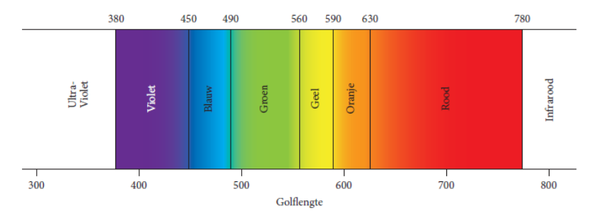
Figure 19-1: The spectral distribution of solar visible radiation (light) with its corresponding colours. The wavelengths of light are expressed in nanometres (nm).
There is also some radiation with wavelength shorter than 400 nm, namely ultraviolet (UV), but this is no more than a few percent of the total at sea level. However, UV radiation is very high in energy and, despite its small share in total solar radiation, can be harmful to plants, humans and animals. Leaves are protected from UV damage by UV-absorbing pigments (such as flavonoids) in the epidermis. This allows less than 1% of UV-B radiation (the most harmful part of the UV spectrum with a wavelength between about 280 and 315 nm) at leaf level to penetrate the mesophyll, which contains the photosynthetic pigments.
At the “red” end of the spectrum, with wavelengths longer than 720 nm, there is still some 40-45% of the sun’s incoming radiation energy. Although this infrared radiation is not visible to our eye and not photosynthetically active, it is energy-bearing and thus warming. This radiation is referred to as near-infrared radiation (NIR) because its wavelength is close to the visible part of the spectrum. There is also far-infrared, but for this the designation ‘long-wave radiation’ or ‘thermal radiation’ is usually used. In practice, short-wave radiation (including near-infrared) comes from the sun, and long-wave radiation comes from terrestrial objects and the atmosphere. The boundary between both forms of radiation is placed at a wavelength of 3000 nm.
19.3 Radiation behaviour in vegetation
19.3.1 Reflection and transmission
Chlorophyll absorbs PAR but not NIR, and therefore the reflection (rebound) and transmission (let-through) of light by green leaves are much greater in the wavelength range of the NIR (above 720 nm) than below. On average, green leaves absorb about 80% in the PAR and 20% in the NIR. The remaining radiation is scattered, either by reflection or transmission. It is therefore understandable that vegetation as a whole reflects radiation much more strongly in the NIR than in the PAR. In the well-known ‘false-colour’ recordings of the Earth’s surface from drone, aircraft or satellites, vegetated surfaces can therefore be easily recognised by their bright red colour, which in fact reflects the NIR colour (Figure 19-2). The reflectance of a single, horizontal leaf is 10% in the PAR and 40% in the NIR. However, leaves are spread out in all directions and overlap each other so that a lot of radiation goes past the leaves. Seen from above, only the upper leaves are in full light, and in between there are dark shadow spots that catch radiation. As a result, by radiation extinction, the reflection of a crop is smaller than that of leaves lying horizontally, i.e., 5% for PAR and 20% for NIR. Through repeated scattering within the crop, the reflectance increases, whereby the correction for NIR is much larger than for PAR. Finally, we then arrive at a reflectance of 5.5% for PAR and 38% for NIR for a homogeneous and dense crop (Goudriaan & Van Laar, 1994).
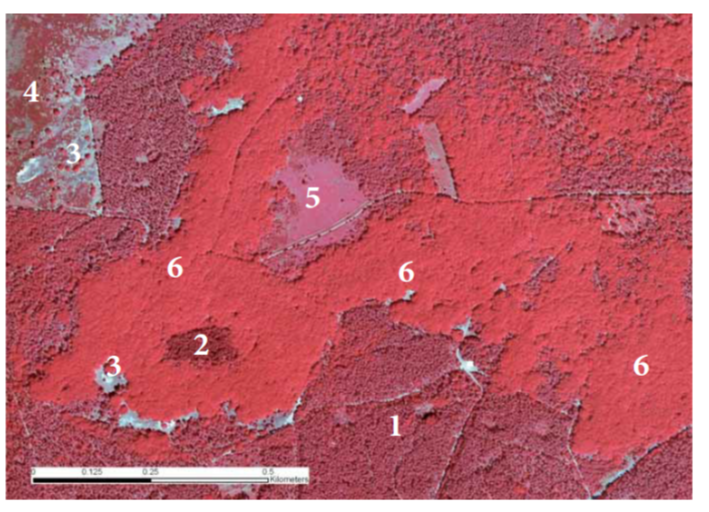
Figure 19-2: False-colour aerial photograph from 2006 of part of the Kootwijk forest reserve near forest reserve Riemstruiken on the Veluwe. This shows the contrasts between the old oak forest, the drift sand afforestation with Scots pine and remnants of drift sand vegetation. Ground cover: 1: drifting sand afforestation with Scots pine; 2: douglas fir forest; 3: drifting sand partly open (white), partly overgrown with buntgrass and lichens; 4: heather on drifting sand; 5: grass dominance (pipe-straw); 6: old oak forest (former coppice). Photo: copyright Eurosense BV DKLN-2006.
In a forest, leaves are clustered much more strongly around branches and trunks than in an agricultural crop. As a result, even more radiation is caught in darker gaps between the trees, and the reflectance coefficient of a forest is still 20 to 30% lower than that of agricultural crops: around 4% for PAR and 30% for NIR.
The albedo is the average reflectance for the entire short-wave region of solar radiation. Because incoming radiation contains about the same amount of PAR as NIR, the albedo is the average of both reflection coefficients, and this works out to about 17% for a forest, compared to 22% for grass or an agricultural crop. A forest thus looks somewhat darker than other vegetation on aerial photographs (Figure 19-2). In winter, of course, the situation is completely different. In a deciduous forest, the leaves are then gone and the reflectance in the NIR region will be much lower, and not much different from that for PAR. In the leafless period, the soil reflectance becomes important, and this in turn depends heavily on the soil type and especially on the humidity of the top layer. A wet soil is much darker than a dry one. The albedo of a bare soil will usually be between 10 and 30%. On the other side, the albedo of fresh snow can reach up to 90%.
In a homogeneous vegetation cover, as in the case of an agricultural crop, the downward decrease constitutes the main variation in light intensity. The vertical gradient is characterised by an exponential decrease in light intensity in function of the overlying leaf area, expressed in LAI (‘Leaf Area Index’). The LAI is determined by the amount of unilateral projected leaf area per unit ground surface, and expressed in m2m-2 (see Table 19-1). The formula for light extinction is:
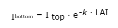
where Ibottom and Itop are the light intensity below and above the canopy, respectively, and k is the extinction coefficient (dimensionless). This formula is known as Lambert-Beer’s law.
In the PAR range, in a homogeneous canopy k is 0.7, with this the light halves with roughly every unit of LAI. In the case of the crown canopy of a forest, as the forest ages, clustering of the leaf canopy around twigs increasingly occurs, grouping of twigs around larger branches, and clustering of branches into tree crowns (see Figures 19-3 and 19-4).
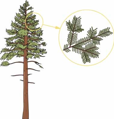
Figure 19-3: Clustering of needles in tree crowns and around twigs.
As a result of this clustering, radiation penetrates deeper into the crown canopy and solar radiation can be distributed over a greater number of leaf layers. Thus, the value for the extinction coefficient in forest is usually lower than for a homogeneous canopy, and it is better to use a value for k of 0.5 for forest. With a lower value for k, the radiation penetrates deeper into the crown canopy and, with equal LAI, the total transmission and thus the light level under the crown canopy will be greater (see Figure 19-5). The value for LAI is determined by the total amount of leaves or needles and depends on the productivity of the growing site. On good growth sites, LAI is higher than on poor growth sites, and shade tree species generally have a higher LAI than light tree species. The total leaf or needle area is correlated with the total area of the active sapwood, as there is a functional balance between the total evaporating area and the area of the transport tissue (pipe model theory). Table 19-1 shows some typical LAI values for different tree species.
Apart from leaves and/or needles, radiation is also intercepted by the surface of trunks and branches. The wood area index (WAI) as perpendicularly projected surface of trunks and branches can reach values of 0.5 – 1.0 m2m-2 in a mature forest in some conditions, and in that case provides an additional transmission reduction of 10-20% (Halldin 1985). In mechanistic models, it is usually assumed that the branch and trunk surface is mostly below the leaf surface, and can therefore be neglected when calculating of total photosynthesis based on light under- creation by individual canopy layers (Mohren 1987).
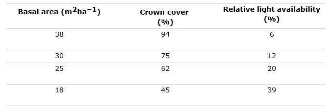
LAI is strongly correlated with the basal area of the tree (in fact: with the sapwood area, see Chapter 13), and with decreasing basal area resulting in decreasing crown cover, transmission and light availability under the crown canopy increase correspondingly (see Table 19-2).
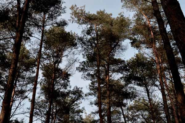
Figure 19-4: Clustering of needles in tree crowns and around branches in a Scots pine forest in Oostereng forest. Photo: Leo Goudzwaard.
Table 19-1: LAI values for a closed forest of different tree species and two agricultural crops for comparison (data from Cannell 1982).

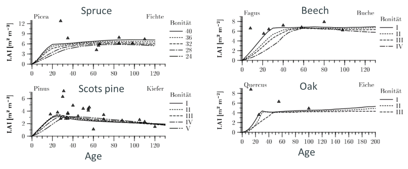
Figure 19-5: Leaf area index (LAI) of different trees species and depending on age (Hörmann et al. 2003)
Table 19-2: Basal area, crown cover percentage and relative light availability as percentage of light above the canopy in a mixed stand consisting of Norway spruce, silver fir and beech in southern Germany (Bavaria) (Grosse, 1983).
In the NIR, the vertical extinction is less because of the smaller absorption by the leaves. A good approximation is that the extinction coefficient for NIR is about half that for PAR, and in a homogeneous canopy thus has a value of around 0.35. This difference in extinction results in a strong shift in spectral composition as we move deeper into the canopy. While incoming sunlight has a PAR-NIR ratio of 1:1, under an LAI of 4 m2m-2 it will have decreased to 1:4. The literature usually uses the term ‘Red-to-Far-Red ratio’ because the decrease in light absorption is most pronounced around 720 nm.
Plants may react strongly to the Red-Far-Red ratio during their elongation growth. A low Red-to-far-Red ratio is a signal for plants that they are in a vegetation and thus have to compete for light. They will respond by investing in height growth.

Figure 19-6: Transmission of radiation through a homogeneous crown canopy, according to e–k∙LAI , with k = 0.3, k = 0.5 and k = 0.7; a combination of k = 0.3 for NIR and k = 0.5 for visible radiation corresponds to the situation in a coniferous forest with clustered needle surface.
Horizontal variation
The clustering of leaves and needles around twigs and branches creates variation in the light climate and this variation generally increases as the forest ages. As an even-aged stand ages, gaps gradually appear in the crown canopy, causing an increasing proportion of radiation to fall directly onto the ground. This is one of the reasons why forest growth declines with age (see Chapter 14). As a result of this variation in the crown canopy, there is considerable horizontal variation in light intensity, especially in hellish weather. At an upper LAI of 1 m2m-2, the average downward PAR is about 50% of the incoming value, but when the sun shines, this average is made up of spots with almost full sunlight and spots with strong shade (Figure 19-6). Those spots with high sunlight receive radiation directly from the sun, i.e., without reflection or scattering. This is referred to as direct radiation. In turn, strong shaded areas receive radiation that is strongly scattered in all directions, which is referred to as diffuse radiation. We also find this divergence of solar and shade patches on the leaves, and because photosynthesis is already saturated well below the intensity of full sunlight, we have to distinguish between shaded and sunlit leaves when calculating tree/forest photosynthesis. Variations in the openness of the crown canopy and the position of the sun lead not only to differences in light intensity, but also in the composition of light reaching the forest floor. This results in a strong differentiation in the undergrowth of the forest, both quantitatively and qualitatively, in light environments to which plants and also animals respond (Endler, 1993, see Figure 14-8).

Figure 19-7: Horizontal distribution of sunlight under an almost closed crown roof of beech. The bright spots are caused by direct radiation hitting the forest floor, shifting continuously throughout the day with the movement of the sun. Between the sunspots, only diffuse radiation falls on the ground. Photo: Jan den Ouden.
The radiation intensity received by vegetation is not constant and varies both over the day and over the year. On a diurnal basis, radiation dynamics depend on the day length on the one hand and the sun’s altitude on the other. Both factors are obviously related to each other (Figure 19-8). The bell-shaped course of the radiation dynamics is typical. During summer, daylength is greater and higher solar altitude means that higher radiation intensity is received compared to the winter period (Figures 19-8 and 19-9). Cloud cover can greatly reduce the radiation intensity, so the amount of radiation received can be very low on cloudy winter days. Cloud cover affects the proportion of diffuse and direct radiation. In the absence of cloud cover, the proportion of direct radiation is highest, while in strong cloud cover there is only diffuse radiation.
On a seasonal basis, the received radiation intensity shows a sinusoidal gradient because of the sinusoidal gradient of the sun’s height in the sky (Figure 19-9). Deviations from a perfect sine wave are due to cloud cover.
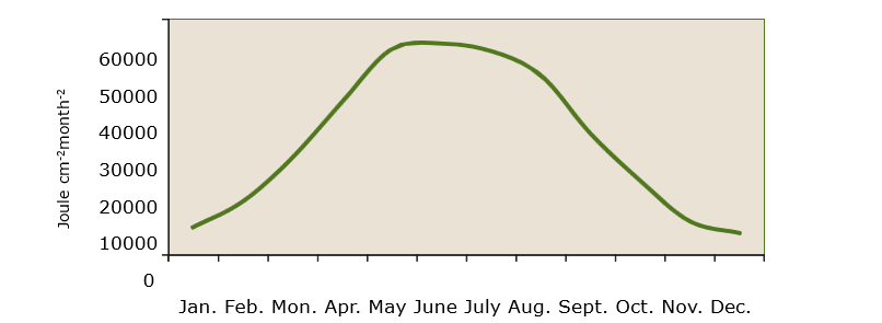 Figure 19-8: The annual course of global radiation at De Bilt, based on average monthly totals (in Joule cm-2month-1 over the period 1961-1990. Data from Krijnen & Nellestijn (1992).
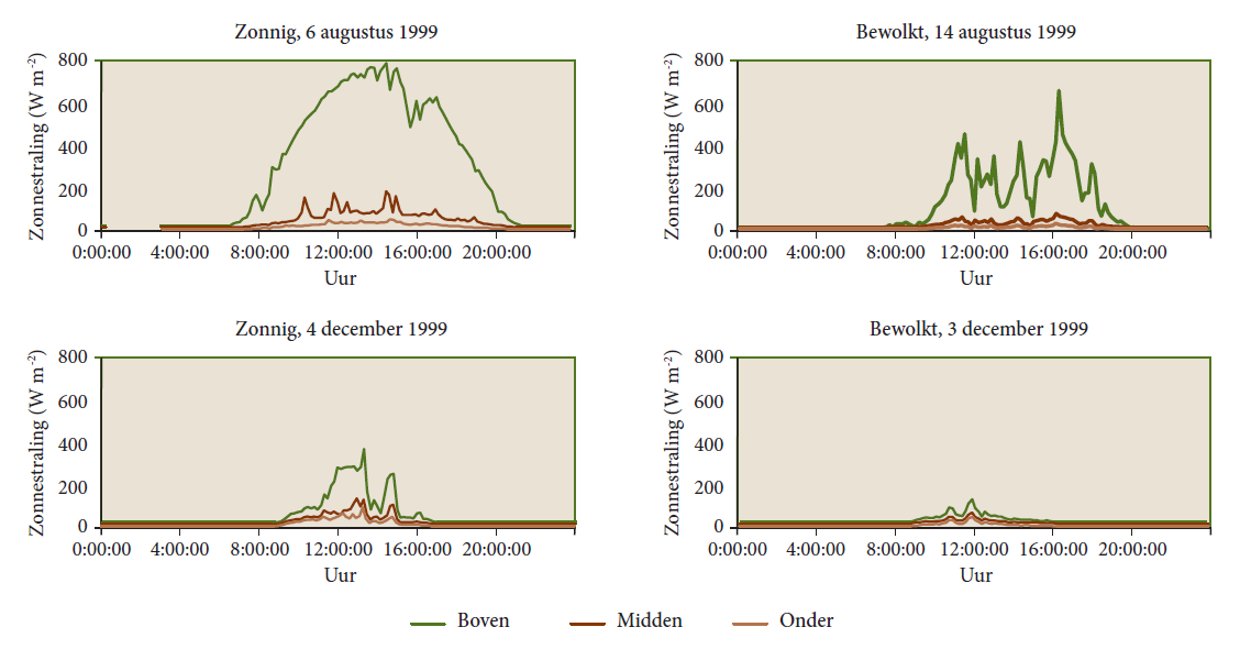
Figure 19-9: Daily course of radiation on two sunny and two cloudy days in August and December respectively, at the Aalmoeseneiebos (Ghent, Belgium). The upper line shows the incoming radiation above the canopy, the middle (dark brown) line gives the radiation directly below the canopy, and the lower line shows the radiation level directly above the forest floor. (Samson 2001).
19.5 Efficiency in radiation conversion
Part of the incident solar radiation, especially PAR radiation, is absorbed by the vegetation and used for photosynthetic carbon assimilation. This conversion into biomass is particularly important in forestry terms. If one wants a first rough approximation of the biomass increase as a function of the actual meteorological conditions (in this case, the amount of irradiation), one may use the Radiation Use Efficiency (RUE, usually expressed in grams of biomass production per Megajoule: MJ, 106J). This expresses how efficiently biomass is produced as a function of incident solar radiation. The theoretical maximum value for RUE is about 3 g MJ-1 (Cannell 1989); in a field situation, Bartelink et al. (1997) give values for above-ground beech production of 1.4-1.5 g MJ-1 and above-ground douglas production of 1.0-1.1 g MJ-1. The concept of RUE is a useful tool in summary models of forest growth (Bartelink et al. 1997).
The units of this variable can vary according to what exactly is considered: total biomass or only above- ground (stem) biomass expressed as fresh or dry weight (tonnes ha-1yr-1), carbon (tonnes C ha-1yr-1), CO2 (tonnes CO2 ha-1yr-1) or energy content (MJ m-2yr-1). Incident radiation (St) is usually expressed in energy units (MJ m-2 yr-1). Factors such as drought stress or nutrient deficiency can reduce this efficiency. To account for these limiting stress factors, one can consider additional reduction factors. The overall formula can then be written as follows:

where εd and εn are the reduction factors for drought and nutrients, respectively. The values of these coefficients range between 0 and 1 (with 1 for no limitation) and are dimensionless. Such reduction factors include sub-optimal growing conditions, such as water and nutrient deficiencies, and are thus in fact also a measure of site index.
19.6.1 Energy balance components
The energy for evaporation, heating and photosynthesis is provided by the net balance of short-wave and long-wave radiation. This net radiation (Rn) can thus be written as follows:
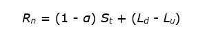
where α is the albedo, St the total (direct and diffuse) incoming short-wave solar radiation, Ld the long-wave (thermal) downward radiation and Lu the long-wave upward radiation.
Since the net radiation above the tallest trees would have to be measured, it is useful to be able to estimate the net radiation from commonly measured solar radiation values by using an empirical expression. Samson (2001) found the following relationship below above a mixed oak-beech forest in Flanders (all in W m-2):
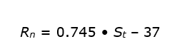
One might expect the coefficient 0.745 in this formula to be equal to 1 – α, but the coefficient is smaller. The additional reduction in net radiation with increasing short-wave irradiance is due to heating of the canopy and consequently increasing upward long-wave radiation. This heating coefficient is of the order of 0.085; with a value for α of 0.17, this gives 1 – 0.17 – 0.085 = 0.745. The constant term -37 W m-2 in the formula represents the thermal radiation loss at night, when St is zero; during the day the loss is larger and this is accounted for in the ‘heating coefficient’ of 0.085. The thermal radiation loss depends strongly on the cloud cover with the extremes being -100 W m-2 for dry and clear weather and -10 W m-2 for heavily cloudy weather (all values in W m-2). Besides the energy for evaporation, heating and photosynthesis, part of the net radiation (Rn) is also used for warming the soil and biomass, especially in the morning. Effectively, this energy is only temporarily stored and released at night or during the winter period (Samson & Lemeur 2001). Usually, this energy storage is simplified to the soil heat flux at a certain (shallow) soil depth (G), while the other terms (such as energy storage in logs) are ignored (Shuttleworth 1994).
The net available energy (Rn -G) is then divided between two processes, namely the sensible heat flux (H) and the evaporative flux (or latent heat flux) (λE):
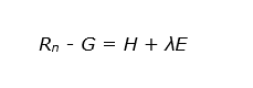
All terms in this equation are expressed as a flux density with units of energy per unit area per unit time (J m-2s-1 or W m-2). The amount of energy consumed in the photosynthesis process is very low compared to net radiation and to latent and sensible heat fluxes (less than 1%), and in micrometeorology usually is accounted for in the storage term G.
Large amounts of energy are exchanged by convection between the surface, in this case the forest vegetation, and the atmosphere. This convective heat exchange between the vegetation and the atmosphere is called the sensible heat flux (H) (Rosenberg et al. 1983).
Very important for forest ecosystems is the energy exchange in the form of evaporation (λE, where E represents the transpiration flux in kg m-2s-1 or mm h-1 and λ the latent heat of water vapour in J kg-1). During evaporation, liquid water is converted into water vapour. This process requires a particularly large amount of energy. On average, on a daily basis, as much as three quarters of the net radiant energy is used for evaporation. We do not feel this energy flux as a change in air temperature, which is the case with the sensible heat flux; hence the name ‘latent (hidden) heat flux’.
As a result of their height, combined with the rigidity of the woody canopy structure, trees and forests are aerodynamically rough. That is, forests can very easily transport energy but also all kinds of particle matter (e.g. CO2, water vapour, N compounds, O3 and fine dust) may exchange with the atmosphere above. We may say that forests are strongly coupled with the atmosphere above. A variety of well-developed micrometeorological methods are available to calculate evaporation from vegetation cover in relation to local weather conditions, surface characteristics and physiological control mechanisms such as stomatal opening and closing. One of the most widely used methods for this purpose is the Penman-Monteith equation (Monteith 1965). Due to the strong coupling of forests to the atmosphere, the Penman-Monteith equation is a good approximation for estimating evaporation by forest ecosystems (Samson & Lemeur 2001). For a more detailed description of the modelling of evaporation and other micrometeorological processes, consult with more specialised publications such as Jones (1992), Goudriaan and Van Laar (1994), Monteith and Unsworth (1990) and Samson (2001).
19.6.2 Energy balance dynamics
The energy balance and its various components show diurnal and annual dynamics influenced by day length and sun height. On a daily basis, as for St, we observe a bell-shaped evolution of net radiation Rn (Figure 19-8). Note that at night and during early morning and late afternoon Rn is negative. This can be explained by the temperature dependence of long-wave components. Since the downward component Ld is dependent on the colder atmosphere (with an approximate height of 10 km and a temperature decrease of -6°C km-1), and the outward component Lu is dependent on earth temperature (with an average temperature of 15°C), the net long-wave term is always negative resulting in loss of energy. Since St at night equals zero by definition, Rn is negative during the night and during early morning and late afternoon. As described above for incoming solar radiation, the net radiation Rn shows a sinusoidal gradient during the year again with deviations from this sinusoidal gradient due to cloud cover.
Energy exchange by evaporation (λE) is especially important in the growing season. The energy not lost via evaporation is lost via the sensible heat flux (H). Note that both the latent and the sensible heat flux can take on a negative value, implying a flow of energy in the opposite direction. In the case of latent heat (λE<0) this indicates condensation of water on the vegetation (dew formation), in the case of sensible heat (H<0) we speak of advection. In advection, additional energy flows sideways into the ecosystem via horizontal air movement. The latter process is of substantial importance in, for example, urban ecosystems (street trees, urban parks, urban forests) and may cause additional evaporation by vegetation. This leads to an improvement of the urban climate (decrease in air temperature) and is also referred to as the ‘oasis effect’.
During winter months, net radiation on a daily basis is very low and may even be negative, limiting both sensible and latent heat exchange. Ecosystems with deciduous trees will show lower evaporation during winter and part of spring anyway due to the leafless state, although evaporation may also occur from the soil and litter layer and on branches and trunks in the form of evaporation of interception water (see Chapter 20).
According to Orlanski (1975) the scale of microclimate is splitted in α-microclimate from a horizontal scale of 2km to 200 m, β-microclimate from 200 m to 20 m and γ-microclimate below. The microclimate of a vegetation refers to the weather conditions inside vegetation, such as in and under the crown canopy of a forest. Climate is the average (over a larger period of time) state of the weather at a particular place. So actually, it would be better to speak of micro-weather precisely because we are concerned with the relationship between the micrometeorological features (weather) above or outside the vegetation and the conditions inside the canopy. Microclimate is less about averages over a longer period of time and more about the instantaneous situation. The main micrometeorological variables are radiation, temperature, wind, humidity and precipitation. Precipitation is discussed in chapter 20 Here, the effect of the canopy on temperature, humidity and wind is briefly outlined. The extinction of radiation in a vegetation cover has already been discussed above: from the top of the crown canopy downwards, radiation gradually decreases, due to interception by leaves and needles, and by other structural elements such as branches and trunks. Especially in forests with high LAI, light levels at the forest floor level can be very low, down to only a few percent of the light level above the crown canopy. As the human eye corrects for the illumination level, the low levels under a forest canopy are not always perceived as such.
As stated before, temperature change is connected with energy balance. The gross energy conversion takes place on surfaces. Thus, there are also the highest changes in temperature. Leafs under direct solar radiation on warm summer days and amplified by drought stress, and limited transpiration, can reach harmful temperatures. Hauck et al. (2025) found that the photosystem II of temperate tree leafs disintegrates between 45 and 50 °C, whereby broadleaved trees were generally more tolerant to heat than conifers.
As a result of the low light levels under a closed crown canopy, net absorbed radiation at the soil surface is low, and only few energy is transformed to soil heat flux and sensible heat, warming up sparsely the air under the crown roof. This means that it remains considerably cooler under the canopy of a closed forest during the day. At night the long-wave upward radiation is lowered by the crown roof, the cooling effect reduced. Thus, the daily variation in temperature is much less pronounced than above the crown canopy (see Figsures 19-10 and 19-11). Under a forest, the air warms less quickly during the day and at night also cools less quickly compared to an open field.
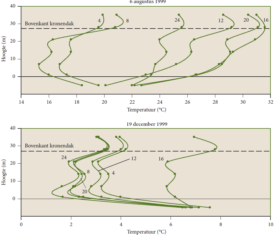
Figure 19-10: Diurnal variation of the vertical profile of air temperature measured at different heights above the forest and in and below the crown canopy, and in the soil in the Alms Grove. The height indicates the distance from the ground level; the soil temperature was measured at a depth of 4 cm, therefore the soil depth is not shown to scale. The measurements refer to a sunny day in August 1999 and a sunny day in December 1999. The numbering of the profile lines represents the time of day, the dots represent measured values (Samson 2001).
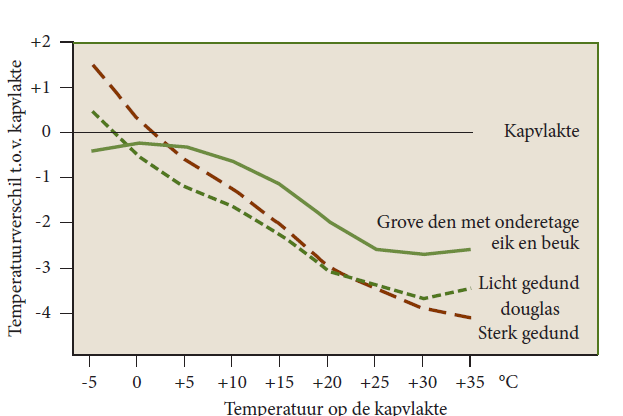
Figure 19-11: The difference in maximum air temperature between three different forest vegetations and a canopy plain without forest near Freiburg (D). Especially at high temperatures, the air in the forest is several degrees cooler. At frost, the douglas-fir forest is warmer. After Mitscherlich (1971).
Besides the radiation driven energy balance, the air movement by advection influences air temperature by surrounded area (see the ‘oasis effect’ above) and topography. At windless, cloudless nights in mountainous regions cool air flows down to valleys and the low temperature can harm sensible trees, although the temperature at the mountainsides remains higher.
Air humidity is the parameter to describe the water vapour content in the air. There are different ways to describe the humidity. The density of water vapour also called absolute humidity gives us the mass of water vapour per air volume in g/m³. As water vapour is a gas amongst others in the air, it is possible to describe humidity with its partial pressure as ea in Pa or mbar. The maximum amount of water vapour in the air, namely the saturated vapour (es) pressure increases exponentially with temperature increase. The relative humidity (RH) is equal to 100 ea / es. With this is the relative humidity also temperature-dependent.
Due to the lower temperature resulting from lower irradiation under the crown roof, RH there is usually significantly higher than above the forest or in the open field (Figure 19-12) and es is lower. The absolute humidity (ea) under the crown roof generally differs little from that in the open field, unless the crown roof is so dense that air exchange is severely restricted. The higher humidity combined with lower temperature makes the microclimate in a forest feel cool on a hot day.
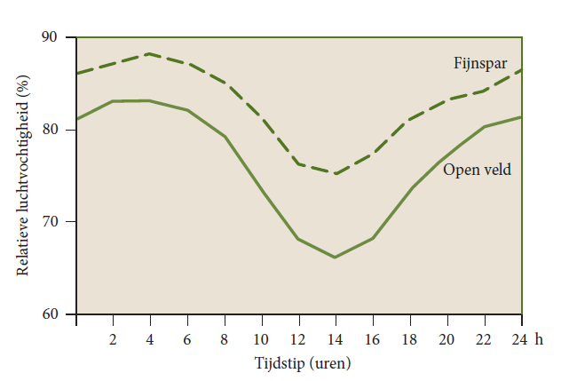
Figure 19-12: The course during the day of relative humidity, averaged over the whole year in a Swiss Norway spruce forest and the nearby open field. In the forest, humidity is always higher. After Mitscherlich (1971).
A driver for evapotranspiration is the vapour pressure-deficit (VPD). VPD is the difference between ea and es. The higher VPD the easier is the water uptake by the atmosphere. At a rH of 100% VPD is 0 Pa. According to the description above VPD increases with increasing temperature, a decreasing absolute water vapour content, or a mixture of both. With increasing temperature by climate change the VPD will exponentially increase.
As with the effects of the crown roof on temperature and humidity, the effect of the canopy on the wind profile, the gradient of wind speed with height, is strongly determined by the density and structure of the canopy. The wind speed decreases directly above the canopy, with the rate of decrease determined by the roughness of the canopy structure (see Figure 19-12). The decrease of wind along canopy height down to a fictitious zero plane somewhere in the canopy can be described by a logarithmic wind profile:
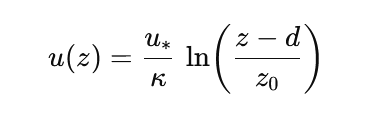
with uz the wind speed at height z in ms-1; u* the friction speed derived from the wind profile, also in ms-1 , k the von Karman constant (k = 0.41); z the height above the ground in m; d the zero plane displacement in m (the imaginary height in the crown roof where the wind speed would be zero if the logarithmic profile above the crown roof were extrapolated uniformly, see Figure 19-12); and finally zo the roughness length in m, a measure of surface roughness that is on the order of 0.1 x the height of the forest. The value for the friction velocity u* is estimated as a regression coefficient from the observed wind profile, based on assumptions about the zero-surface displacement d (e.g., d = 0.7 x tree height) and the roughness length zo (e.g., as 0.1 x tree height). The wind profile above the forest is determined by the aerodynamic roughness of the forest, and from the wind profile it can then be deduced how fast perceptible and latent heat are dissipated to the atmosphere e.g., by calculating an aerodynamic transport resistance that can be used in evaporation calculations such as the Penman-Monteith equation (Allen et al. 1998). Due to the greater surface roughness of forest, the wind speed above the forest decreases faster than in the open field, and exchange is more efficient. Among others, this leads to relatively quick evaporation of rainfall intercepted by the canopy (see Chapter 20).
Under the crown canopy, wind speed is significantly lower than above the canopy (see Figure 19-13), so the exchange of air under the crown canopy with the atmosphere is much less than the air inside the crown canopy itself. The wind speed inside the crown canopy near the virtual zero plane d, is the lowest; it increases again in the free space below the crown canopy, where fewer obstacles such as branches and leaves hamper air movement.
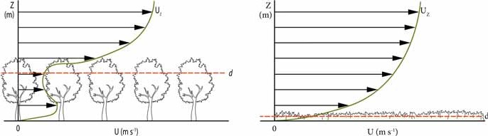
Figure 19-13. Course of wind speed. Left: Course of wind speed with height in a deciduous forest (after Erisman & Draaijers 2003). Right: Progression of wind speed with height above short vegetation. The decrease in wind speed with height is much smaller, down to close to the ground. d: fictitious zero surface displacement
The final result of all these effects together – temperature, radiation, humidity and wind – leads to the conditions under the crown canopy being much more moderate than above or in the open field, and hence extremes are attenuated. This thus provides conditions in which regeneration of especially shade-tolerant tree species can establish and develop.
19.8 Synthesis: Effects of trees and forests on microclimate
Depending on their type (coniferous forest, deciduous forest), structure (horizontal and vertical forest structure) and form of use (e.g., age-class forest with clear-cutting regeneration vs. continuous-cover forest), forests can decline radiation and buffer (extreme) temperatures and thus influence the internal forest climate. Shading and evaporative cooling through increased evapotranspiration are decisive factors here (Mitscherlich 1981).
Von Arx et al. (2012) measured temperature differences of up to 5 °C (daily maximum air temperature) in stands with intact crowns compared to open areas on permanent observation plots in Switzerland. The air humidity in the stands with canopy cover was also higher than in stands without canopy cover. The greatly reduced wind speeds inside relatively closed stands can contribute to slower removal of moist air parcels and thus reduce evaporation. The microclimatic buffering effect of the forest against extreme weather was particularly pronounced in shade-tolerant deciduous and coniferous forests, but comparatively low in pine forests (von Arx et al. 2012).
The extent of canopy openness in forest regeneration and its effect on temperature buffering is therefore increasingly being discussed. In particular, small-scale selective cutting or gap cutting (e.g., with a ratio of gap diameter to tree height of the surrounding stand ≤ 1) leads to only a slight increase in temperature in the gap (Mitscherlich 1981). Thom et al. (2023) measured a temperature difference of 1.9 °C between clear-cuts and a stand with intact canopy cover in the Bavarian Forest during the summer months, with a gap size of 625 m². A comparison of the buffering effect of a pine and beech forest on the Britz intensive monitoring area of the Thünen Institute in Eberswalde showed that the beech forest has the fewest hot days and the average temperature on hot days is lower there (Thater 2023). Above all, the air temperature near the ground is better buffered as temperatures rise, especially in beech forests.
When analysing stand structure parameters, canopy opening has the greatest effect on the temperature buffering effect (Frey et al. 2013; Ehbrecht et al. 2019). In contrast, tree species diversity has only a marginal direct effect on the forest microclimate (Gillerot et al. 2022). A study from Berchtesgaden National Park shows that the buffering effect of temperature extremes is particularly high during the establishment and optimal phases, while gaps, terminal and decay phases are warmer (Sieblitz 2023). This indicates a rapid recovery of the forest interior climate after small-scale disturbances. Moreover, with respect to regeneration this points out to the urgent need to keep canopy openings as small as possible, especially in beech stands.
Global studies also confirm this moderating effect of the forest canopy (Zellweger et al. 2020; de Frenne et al. 2019). A closed canopy buffers strong macroclimatic changes and slows down changes in the species composition of the ecosystem, while large gaps in the canopy accelerate change. This buffering effect appears to increase as temperature extremes become more pronounced.
References
Allen, Richard G., Pereira, Luis S., Raes, Dirk, Smith, Martin (1998) – Crop evapotranspiration – Guidelines for computing crop water requirements – FAO Irrigation and drainage paper 56 – Part A, Chapter 2 – FAO Penman-Monteith equation. FAO – Food and Agriculture Organization of the United Nations; Rome; https://www.fao.org/4/x0490e/x0490e06.htm#fao%20penman%20monteith%20equation
Arx, G. von, Dobbertin, M., Rebetez, M. (2012). Spatio-temporal effects of forest canopy on understory microclimate in a long-term experiment in Switzerland. Agricultural and Forest Meteorology 166-167, 144–155.
Ehbrecht, M., Schall, P., Ammer, C., Fischer, M., Seidel, D. (2019). Effects of structural heterogeneity on the diurnal temperature range in temperate forest ecosystems. Forest Ecology and Management 432, 860–867.
Erisman & Draaijers 2012. Moving forward with forest governance, ETFRN news; issue no. 53. Wageningen: Tropenbos International.
De Graaf, L., 2012. “Communication about medications for better patient transition. Needed: Format for switching.” Pharmaceutisch Weekblad no. 147 (8):14-15.
Fernandes, Alvaro A. A., Alasdair J. G. Gray, and Khalid Belhajjame, 2011. Advances in Databases: 28th British National Conference on Databases, BNCOD 28, Manchester, UK, July 12-14, 2011, Revised Selected Papers. Berlin, Heidelberg: Springer Berlin Heidelberg.
Frenne, P. de, Zellweger, F., Rodríguez-Sánchez, F., Scheffers, B. R., Hylander, K., Luoto, M., Vellend, M., Verheyen, K., Lenoir, J. (2019). Global buffering of temperatures under forest canopies. Nature Ecology & Evolution 3/5, 744–749.
Frey, S. J. K., Hadley, A. S., Johnson, S. L., Schulze, M., Jones, J. A., Betts, M. G. (2016). Spatial models reveal the microclimatic buffering capacity of old-growth forests. Science Advances 2/4, e1501392.
Gillerot, L., Landuyt, D., Oh, R., Chow, W., Haluza, D., Ponette, Q., Jactel, H., Bruelheide, H., Jaroszewicz, B., Scherer-Lorenzen, M., Frenne, P. de, Muys, B., Verheyen, K. (2022). Forest structure and composition alleviate human thermal stress. Glob Change Biol 28/24, 7340–7352.
Hauck, M., Schneider T., Samuel Bahlinger, Judith Fischbach, Gabriella Oswald, Germar Csapek, Choimaa Dulamsuren (2025) Heat tolerance of temperate tree species from Central Europe, Forest Ecology and Management, 580, doi.org/10.1016/j.foreco.2025.122541
Mitscherlich, G. (1981). Wald, Wachstum und Umwelt – Eine Einführung in die ökologischen Grundlagen des Waldwachstums. 2. Band – Waldklima und Wasserhaushalt. J. D. Sauerländer‘s Verlag, Frankfurt am Main.
Orlanski, I. (1975) A rational subdivision of scales for atmospheric processes. Bull. Am. Meteorol. Soc. 56:527-530Sieblitz, F. (2023). Der Einfluss der Bestandesentwicklung auf das Waldinnenklima im Nationalpark Berchtesgaden. MSc-Thesis. TU München.
Thater, N. (2023). Stand-level microclimatic effects of Fagus sylvatica and Pinus sylvestris in relation to open land between 2018 and 2022 at the Ecological Research Station in Eberswalde Britz. Bachelor Thesis. HNE, Eberswalde.
Thom, D., Buras, A., Heym, M., Klemmt, H.-J., Wauer, A. (2023). Varying growth response of Central European tree species to the extraordinary drought period of 2018‐2020. Agricultural and Forest Meteorology 338, 109506.
Zellweger, F., Frenne, P. de, Lenoir, J., Vangansbeke, P., Verheyen, K., Bernhardt-Römermann, M., Baeten, L., Hédl, R., Berki, I., Brunet, J., van Calster, H., Chudomelová, M., Decocq, G., Dirnböck, T., Durak, T., Heinken, T., Jaroszewicz, B., Kopecký, M., Máliš, F., Macek, M., Malicki, M., Naaf, T., Nagel, T. A., Ortmann-Ajkai, A., Petřík, P., Pielech, R., Reczyńska, K., Schmidt, W., Standovár, T., Świerkosz, K., Teleki, B., Vild, O., Wulf, M., Coomes, D. (2020). Forest microclimate dynamics drive plant responses to warming. Science 368/6492, 772–775.
Acknowledgements
This Chapter is published on the EUROSILVICS platform, established as part of the EUROSILVICS Erasmus+ grant agreement No. 2022-1-NL01-KA220-HED-000086765.
This text is largely based on Ch 9 “Radiation and Energy balance” from the Dutch textbook “Forest Ecology and Forest Management”, written by R. Samson, J. Goudriaan and F. Mohren.
Author affiliation:
| Frits Mohren | Wageningen University and Research, Wageningen, The Netherlands |
| Marco Nathkin | Von Thünen Institute, Eberswalde, Germany |
| Peter Spathelf | Eberswalde University for sustainable development, Germany |