
Chapter 14: Tree and Forest Growth – Download PDF
Authors: Bart Muys, Jan den Ouden, Kris Verheyen, Monique Weemstra, Frits Mohren
Intended learning level: Basic
This material is published under Creative Commons license CC BY-NC-SA 4.0.
| Purpose of the chapter: |
|---|
| This chapter introduces the basic principles of growth in trees and forests. |
14.7.1 From tree increment to stand growth 22
14.7.2 Yield class and increment prognosis 22
14: Tree and Forest Growth
Growth is the increase in biomass or in the dimensions of a tree or stand. Sugars produced during photosynthesis are converted into structural biomass and allocated to leaves or needles, branches, stem and roots. Subsequent cell division and cell stretching in meristem tissues leads to increase in biomass and size of the tree. Meristems are tissues of undifferentiated cells capable of cell division, after which these cells develop into other tissues. In the apical meristem, this results in height growth; in the cambium or lateral meristem, this leads to growth in thickness of the stem, branches and roots, mainly due to the formation of xylem tissue (see Chapter 12). The allocation of biomass generally follows a specific morphogenetic growth pattern and determines the habitus (shape) of the tree. Tree growth is the driving force behind stand development, so understanding growth in all its aspects is crucial.
In the first stages of growth a tree primarily invests in height growth (primary growth), and in later stages, diameter growth becomes dominant (secondary growth). From an evolutionary perspective, this pattern can be explained by the fact that a tree has an advantage in first bringing its leaves into a favourable position to intercept sunlight, i.e. above the surrounding plants. Next, the tree needs to develop a solid stem to maintain the acquired position in the canopy and to carry the weight of the developing crown.
The growth rate of a tree depends on its genetic predisposition (species or provenance; see chapter 17), temperature and radiation, and the availability of water and nutrients (site quality; see chapter 18). Within a forest stand with homogeneous site conditions where moisture and nutrients are in ample supply, individual tree growth will be primarily determined by the available light, and will therefore be proportional to the tree’s share of light interception. The consequences of this for the interactions with neighbouring trees (e.g. competition) are further elaborated in Chapter 16. In this chapter, only global patterns in stem height, diameter and volume growth, and root growth will be described, including variation in growth due to differences in site quality.
Height growth results from cell division and cell stretching in the apical meristem, located in the terminal bud of the main axis of the tree (see 12.7.1). Depending on the genetically determined branching pattern, and in interaction with environmental factors, tree shapes develop differently. Monopodial growth occurs in tree species where a single continuous axis extends its apex and produces successive lateral shoots from side buds. This may result in a monocormic crown consisting of a central straight stem (monopodium) with more or less distinct branch whorls around the stem, as seen in most conifers. In other cases a polycormic crown develops, where the central stem gradually dissolves into a branched crown with an irregular structure, as seen in many broadleaved species like maples or ashes (fig. 14-1).
Sympodial growth occurs in tree species in which the main axis is made up of successive secondary axes, like in beech or elm trees. This always results in polycormic crowns (fig. 14.1). From an evolutionary point of view, sympodial growth is advantageous as it offers flexibility to position leaf tissue at any point in the three-dimensional crown space and may thus maximise the use of available light. It is therefore common in shade tolerant species. Forest management that focuses on timber production often prefers conifers because their monopodial architecture produces long straight stems that are easier to harvest, delimb, and process mechanically.
The upper crown parts of trees within a forest stand tend to shade the lower living branches, causing them to die due to lack of light. Such dead branches may detach from the stem (also called self-pruning) and as diameter growth continues a branch-free bole may eventually develop below the living tree crown. In general, self-pruning is more common in broadleaved trees than in conifers, so that conifers receive stem pruning interventions more often than broadleaved species (see chapter 44).
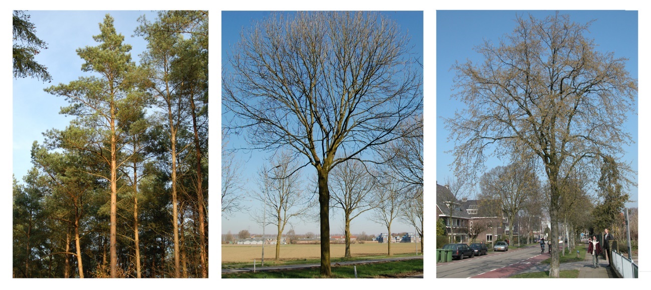
Figure 14-1: Different tree shapes resulting from different branching patterns. On the left a Scots pine (Pinus sylvestris), with clear monopodial growth and strong apical control, resulting in a monocormic stem and crown. In the middle a Common ash (Fraxinus excelsior) with monopodial growth but weaker apical control and frequent mortality of the apex, resulting in a polycormic crown. On the right a hornbeam (Carpinus betulus) with sympodial growth: mortality of branches as a result of shading (and pruning) has created a monocormic stem base, but higher along the stem a polycormic crown has formed without a clear central axis (see also 12.7). Photos Leo Goudzwaard.
Height growth depends on temperature and moisture availability and exhibits periodicity at different time scales. The diurnal (daily) periodicity differs between species. Some species mainly grow at night, while others show a period of rapid growth during the day and a period of slow growth or rest during the night (Mitscherlich 1978; fig. 14-2). The daily height growth rate of a tree is in the order of millimetres to centimetres.
Also the annual periodicity in height growth is strongly species dependent (see fig. 14-3). Species with an outspoken rhythmic height growth, such as oak, beech, pine, spruce and silver fir, have a short concentrated height growth period of only 4-6 weeks in spring, while other species continue to grow in height for most of the growing season, such as hornbeam, poplar, willow, birch, black locust, douglas fir and larch. In years with favourable weather conditions, species -especially from the first group- may form a second or even a third shoot in the summer or fall (see box 14-1: Lammas shoots). The annual increase in height is in the order of decimetres to meters. Especially shoots emerging from a stump may grow several meters in the year following tree felling.
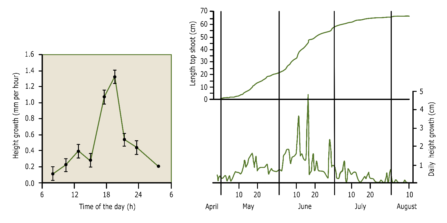
Figure 14-2: Diurnal and annual periodicity of height growth. Left: Typical diurnal pattern of height growth in peach (Prunus persica) growing in optimal conditions. Each point is the average of 5 top shoots. After Berman & De Jong (1997). Right: Height growth of a douglas fir (Pseudotsuga menziesii) during the year, expressed as daily height growth (lower part) and the accumulated height growth over the year (upper part). After Mitscherlich (1978).
Height growth shows different phases during the life of a tree. Height growth increases sharply after seedling establishment, reaches a maximum after a few years to decades and then slowly decreases again (fig. 14-3 and 14-5). The peak in height growth is referred to as the height growth culmination point. Mathematically, the cumulative height curve over time represents the sum of the annual height growth over the entire age of the tree. Inversely, the annual height growth curve shows the derivative or slope of the cumulative height curve at a given tree age. The cumulative height curve typically has an S-shape, where its inflection point corresponds to the culmination point of the annual height growth curve. The timing of the culmination point of height growth is largely species-dependent and, within the same species, is achieved earlier on fertile sites (fig. 14-3).
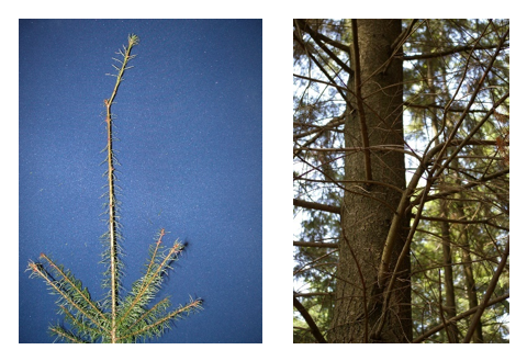
For some coniferous species, like most Pinus species, the annual height increment can be directly inferred from the distance between the successive annual branch whorls, because they develop only one long internode annually (fig. 14-10). At higher ages, total tree height tends to reach a maximum, mainly determined by species and by site conditions, like soil fertility, water availability or air humidity (see chapter 13). When a tree has reached its maximum height, this does not mean that height growth itself has stopped: in such trees a top shoot may form every year, but the top section of the tree regularly dies off, after which height growth is taken over by a side branch to produce the new top.
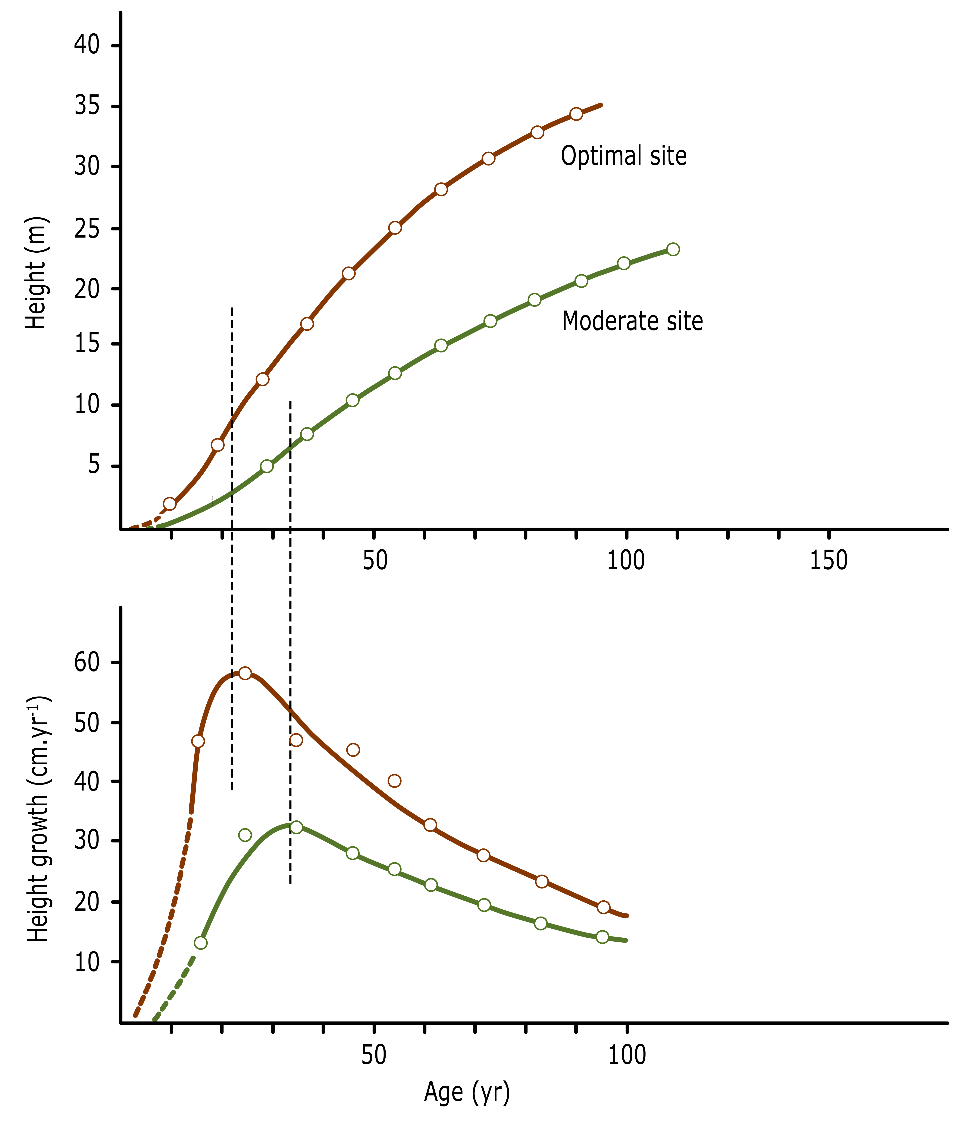
Figure 14-3: Height growth of Norway spruce (Picea abies) at an optimal and moderate site. The culmination point (maximum) of the height growth curve (lower pane) corresponds to the inflection point in the height curve (upper pane) and is more likely to occur earlier in trees at the better sites (here around 23 years) compared to trees at moderate sites (here around 34 years). After Assmann (1961).
| BOX 14-1 Lammas shoots (ADVANCED LEVEL) | ||
|---|---|---|
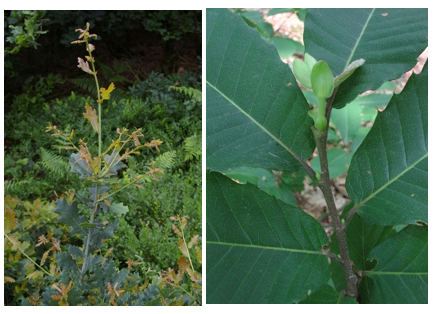
Lammas shoots develop when the newly formed buds of the spring shoot sprout later on during the same growing season (Figure B4-1-1). In some regions these extra shoots are called Saint John’s shoots as in the case of oak this second flush used to appear around June 24, the day of St. John. Under the current, warmer climate conditions, this second flush already occurs early June. In favourable weather conditions, a third, and sometimes even a fourth shoot may occur during the course of summer. In Douglas fir and Scots pine, lammas shoots only occur in late summer.
Figure B14-1-1: Lammas shoots on pedunculate oak (left) and sweet chestnut (right). Photos Jan den Ouden. A majority of the deciduous and coniferous species develop lammas shoots. In pedunculate oak, chances the frequency of lammas shoots occurrence decreases with the size of the increasing tree size. Mature trees only make lammas shoots incidentally in their crown, although in some years with favourable conditions oak may turn red in early summer due to formation of lammas shoots. Seedlings of oak almost always develop lammas shoots. Lammas shoot occurrence is partly genetically fixed and essentially involves breaking bud dormancy. In the case of oak, the lammas shoots are usually longer than the first shoot formed in spring. The lammas shoots thus act as an insurance policy against massive insect herbivory in spring, as in spring not all reserves are will be invested into one extension shoot, with the risk of losing it all to herbivory. The formation of an extra shoot in summer leads to more photosynthesis and shoot extension, but it also poses a risk to the tree. In case the lammas shoot is produced late in the season, damage from early frosts may occur if the shoot has not yet sufficiently hardened. The leaves on lammas shoots of e.g. oak are also susceptible to attack by mildew (Microsphaera alphitoides) due to the large number of mildew spores in the air at the time of the lammas shoots development. Because the lammas shoots are on average longer than the spring shoot in young oaks, a severe mildew infestation can lead to a sharp reduction in height growth and therefore to a reduced competitive position. This is one of the reasons why natural regeneration of oak often has a competitive disadvantage in comparison with other species. As in the case of oak, lammas shoots in Douglas fir are susceptible to fungal infestations. Especially in dense young stands, the lammas shoots may die in large numbers because of encroachment by Botrytis cinerea. The spring shoots are rarely killed by this fungus. Lammas shoots may also lead to large knots in douglas fir, when lammas shoots originate from a side bud, and in the next growing season extend vertically parallel to the top shoot (Fig. B4-1-2). These two shoots can then grow together for a number of years, after which the top shoot may regain apical control. The initially orthotropic growing lammas shoot then suddenly starts to grow plagiotropic and continues to behave like a regular side branch. The result of this is that the lammas shoot is attached to the stem at a very sharp angle and causes a large knot when the tree thickens. This is very unfavourable for wood quality.
Figure B14-1-2. The creation of a double top shoot by the formation of lammas shoot in Douglas fir. The pictures show a lammas shoot adjacent to a lateral bud (left), and a Douglas fir on which a lammas shoot has grown for some time in parallel with the final shoot (right), after which the direction of extension has been deflected and the branch continued to grow as a horizontal side branch. Photos: Jan den Ouden. |
Differences in height growth result in rapid differentiation between different species within mixed stands (Fig. 14-4) and between individuals of the same species within monocultures (see chapter 16). In their first years, species or individuals with inherently rapid height growth are able to quickly acquire a favourable position in the developing canopy. For example, fast growing pioneer species such as larch and birch may be more than one meter higher than potentially competing species within only a few years, allowing these light-demanding species to grow in a mixture with shade-tolerant species that have slower growth. When establishing mixtures of light-demanding species, it is important to choose species that have an approximately equal course of height growth (Jager & Oosterbaan 1994).
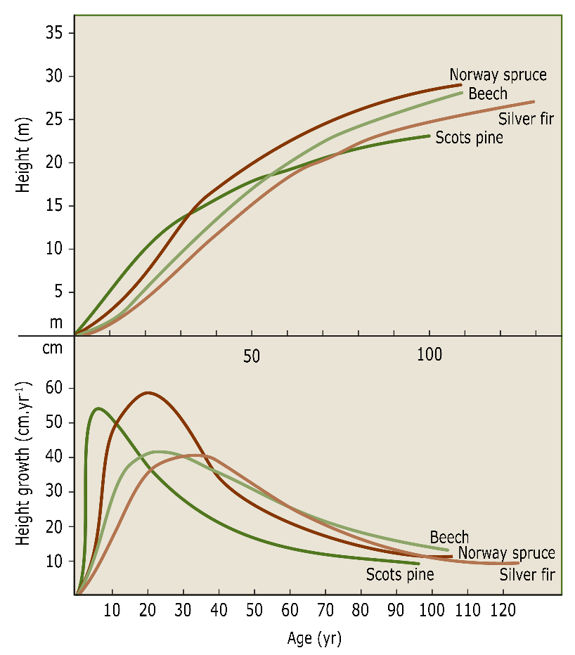
Figure 14-4: Cumulative height and height growth curves for Norway spruce (Picea abies), beech (Fagus sylvatica), fir (Abies alba) and Scots pine (Pinus sylvestris) on the same site. After Assmann (1961).
Height growth in forest stands is usually measured by periodic recording the height of the tree population (the stand) or a particular subset of individuals within the stand. The variables mostly used are the average height, the quadratic mean height, the top height and the dominant height of a stand (definitions in Table 14-1). In homogeneous, even-aged stands, the dominant height or top height is hardly dependent on the tree density of the stand, and is mainly determined by site quality. For this reason, at a certain known age the dominant height or top height of a stand can be used as an indicator of the growth potential (yield class or site class) of a species (fig. 14-15). In very dense stands, however, height growth may be somewhat lower due to intense competition for water and nutrients between individuals. When differentiation in height between individuals is low, high mortality may occur (fig. 14-6). Also in very open stands, the height growth may decrease because total growth is distributed over many terminal meristems on side branches of a larger crown mantle receiving direct light.
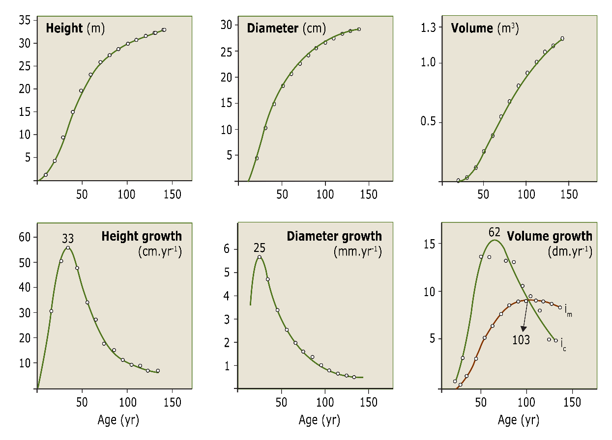
Figure 14-5: Courses of height, diameter and volume growth in time of a Norway spruce (growth curves in lower panes, cumulative growth curves in upper panes). The numbers on top of the growth curves indicate the age of increment culmination. The volume increment (bottom right) is shown both as current periodic increment (Ic; see Table 14-1) and mean periodic increment (Im). After Assmann (1961).
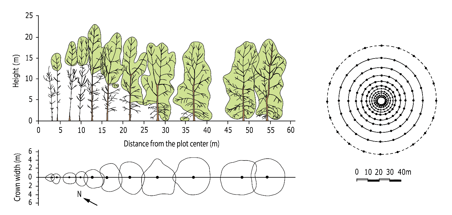
Figure 14-6: Transect drawing from a 14-year-old Nelder experiment with planted poplars (Populus x interamericana ‘Rap’) growing up in different densities. In a Nelder design, the available growing space per tree increases gradually from the centre to the edge of the circular plot. Side view (above) and crown projections (below) along one of the radii of the experiment (right). After Houtzagers & Schmidt (1994).
Table 14-1: Common variables characterising tree dimensions and tree growth, and their aggregate values at the stand level. See also fig. 14-7. After Jansen et al. (2018).
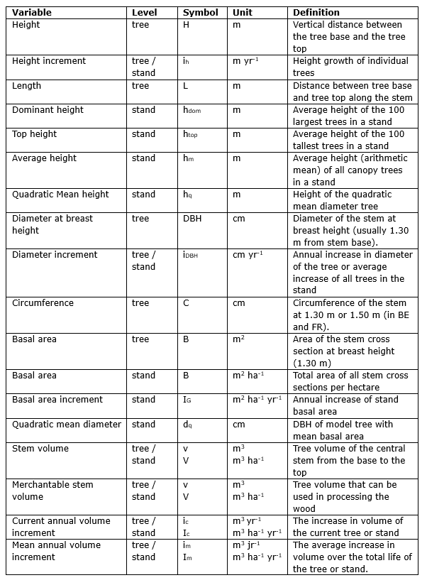
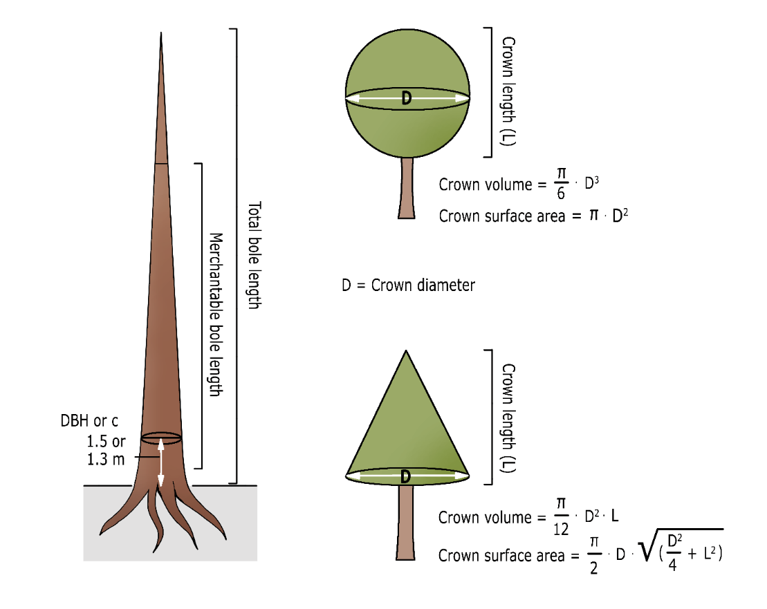
Figure 14-7: Some commonly used measures for determining tree dimensions with geometrical crown shapes.
Diameter increment is the result of cambial activity in which new xylem and bark tissues are formed. In temperate and boreal regions, the seasonality of xylem growth leads to the formation of annual rings, in which earlywood is formed in spring and latewood in summer (see 12.3). After an initial increase, during the juvenile growth phase of the tree, the diameter growth gradually decreases again. As with height growth, this leads to a peak in annual diameter growth (fig. 14-5). This culmination point is usually reached later as compared to height growth. With increasing stand density (crowding) and degree of shading, the culmination point in diameter growth shifts to a higher age. In practice, there is a large variation in diameter growth at a given age due to variation in environmental factors. When a tree grows up in the shade and later becomes exposed to full sunlight, the diameter growth may increase sharply, even when the tree is relatively old. Several periods with higher diameter growth may also occur, causing multiple peaks in the diameter growth curve. This is the case, for example, when a subcanopy tree undergoes several periods of light exposure as a result of thinning or death of surrounding trees.
There are several reasons why, as a rule, diameter growth decreases with tree age. First, when volume growth remains the same, the xylem produced has to be distributed over an increasingly longer and thicker stem, so each layer of new xylem tends to get thinner. Second, a tree maintains a functional balance between the water transport tissue (the xylem) and the foliage biomass. Given a certain transport capacity, a thinner ring of xylem is required with increasing diameter for maintaining the same surface area of conducting tissue. In most species the central heartwood is not functional anymore so no respiration costs are associated with it.
Diameter growth mainly depends on the canopy space available to a tree and the amount of sunlight intercepted by the foliage, and is therefore primarily related to stand density (see table 14-2 and fig. 14-8). With high stem density, and hence limited available growing space per tree, diameter growth is significantly lower than in stands of the same age with a lower stem number. Therefore, site productivity cannot be directly deduced from tree size, and reducing stem density by thinning is a very effective means to stimulate diameter growth (Savill & Sandels 1983; Balleux & Ponette 2006).
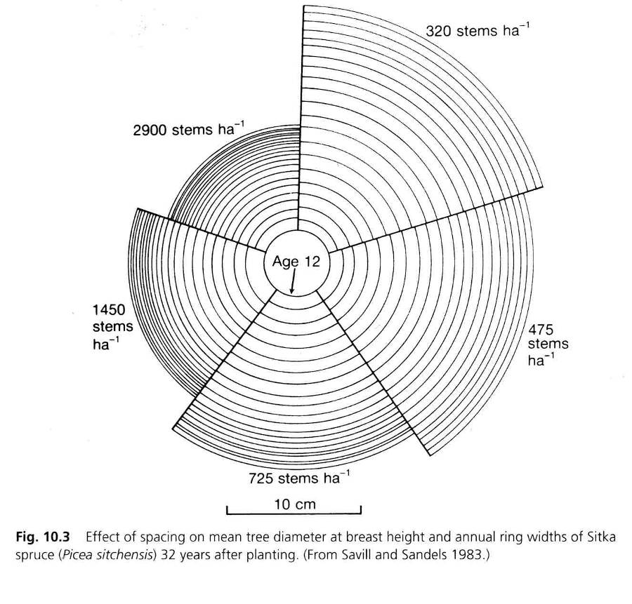
Figure 14-8: The effect of variation in growth space on the DBH growth of Sitka spruce in Great Britain. The trees have grown up to an age of 12 years in the same density (2900 ha-1). Then, several densities were created by a single thinning intervention, after which the trees were felled at the age of 32. After Savill & Sandels 1983.
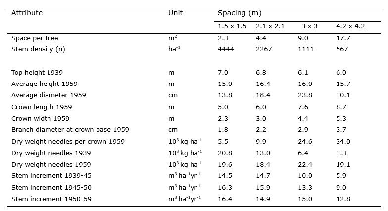
Table 14-2: Influence of the planting density (square planting) on tree characteristics and stand growth in unthinned Pinus ponderosa in North America. The stand was measured in 1939, 1945, 1950 and 1959 and was 17 years old at the start of the measurements (Stiell 1966).
The stem diameter shows clear diurnal variation during the growing season. This is caused by variation in water content, caused by changing water tension within the xylem. During the day, with high water transport and high tension, the stem may shrink slightly. When transpiration stops during nighttime and the water reserves in the stem are replenished, the stem diameter expands again. In drought periods the water content of the stem may also decrease, causing a temporary shrinking of the stem until rains increase water availability again (fig. 14-9). The radial (diameter) growth in a year is determined by the length of the growing season, and of course the soil and weather conditions (Etzold et al. 2022).
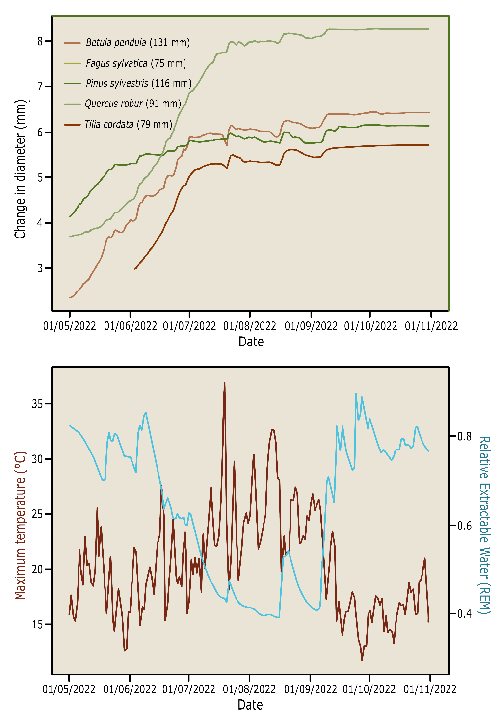
Figure 14-9: Cumulative daily diameter growth, measured by point dendrometers, in Betula pendula, Fagus sylvatica, Pinus sylvestris, Quercus robur and Tilia cordata during the dry growing season of 2022. The lower pane shows the daily maximum temperatures and relative extractable water content of the soil. Data from the tree diversity experiment FORBIO Zedelgem, Belgium.
Diameter growth is not the same along the axis of the stem. In a tree, smaller annual rings are formed at the base of the stem compared to higher positions along the stem (fig. 14-10). Over a year, diameter increase is largest in the lower part of the living crown where the amount of available assimilates is highest, and diameter increase is smallest at the base of the trunk. This differentiation in diameter growth along the stem ensures that the central stem does not develop into a cone, but that a very gradually tapered, more cylindrical shape is formed. Tree species may vary in stem shape, and the pattern in which the stem diameter decreases with height is referred to as taper (see Box 14.2 on bole shape and stem volume).
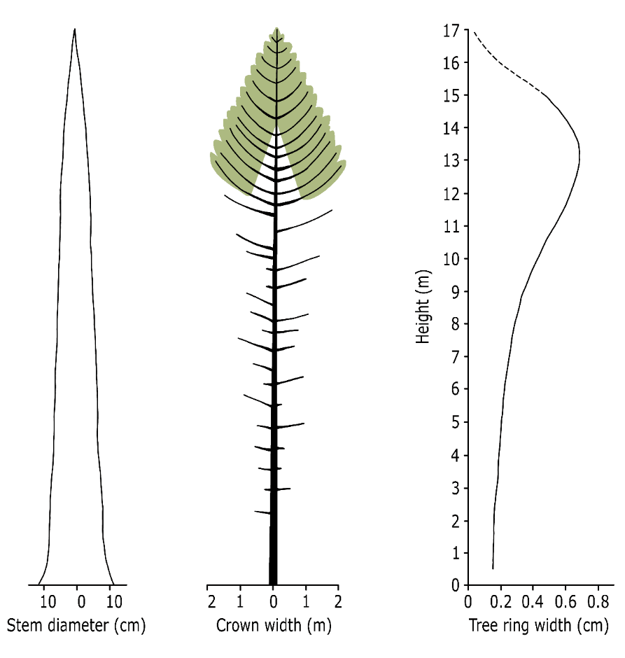
Figure 14-10: Stem shape (left), habitus (middle) and the relationship between tree height and the average annual diameter increase over the last five years (right) in a 38-year-old dominant Scots pine in an unthinned stand (unpublished data, Wageningen University).
Diameter growth can be determined by regular remeasurement of stem diameters at a reference height. In some countries, circumference rather than diameter is measured. The stem diameter or circumference is measured at a standard height from the stem base: the diameter or circumference at breast height or DBH. In most countries, DBH is taken at 1.3 m above the forest floor. Exceptions are, amongst others, Belgium and France, where the stem is traditionally measured at a height of 1.5 m. Repeated measurements in permanent plots are typically done every five or ten years.
The annual increase in height and diameter leads to an increase in stem volume. This volume growth is referred to as increment, and for a single tree expressed in dm3yr-1 or m3yr-1. The increment is usually not considered at the tree level, but rather at the stand level. The current annual increment (Ic or CAI) is the actual growth in m3 ha-1 yr-1. In the case of permanent plots, this is often expressed as periodic annual increment (PAI) in m3ha-1yr-1 calculated as the volume increase over the most recent observation period (e.g. the last five years). The mean annual increment (Im or MAI), is the total increment calculated over the total stand age up to date, including the stem volume removed by thinning over that period (fig. 14-11). CAI, PAI and MAI are concepts developed for even-aged stands, but can be used for uneven-aged forests as well. The volume increment of an individual tree culminates at a higher age than the diameter growth (fig. 14-12).
| Box 14-2: Tree shape and stem volume |
|---|
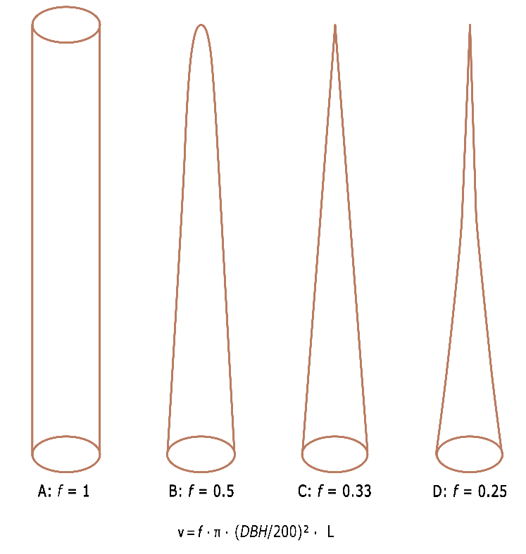
The shape of a tree stem determines the total volume, strength properties, and quality of the sawtimber. The shape also partly determines a number of physiological processes such as water transport. The volume of a tree stem is usually calculated from the stem length or tree height (h, in m), and the thickness or diameter (d, in cm), o0f better the basal area (BA, in cm2) of the stem at some reference height. To accurately determine stem volume, felled trees can be divided into sections of 1-2 m. For each section, it may be assumed that the diameter decreases proportionally with the length of the stem part (section), and that the section has the shape of a truncated cone. The volume of such a stem section i can then be estimated according to Huber’s method as vi = bami · Li, where bami is the mean basal area in m2 of the i-th stem section, calculated as ϖ · ((d1+d2)/400)2) in which d1 and d2 are the diameters of the section ends, and Li is the length of the stem section. The total volume can be obtained by summation of the section volumes. If the shape of a stem strongly deviates from a cylinder, it is desirable to measure many sections to make the measurement error as small as possible. For standing trees, stem volume may be estimated directly from DBH and total tree height. To obtain the correct volume, a correction must be made to allow for the deviation of the stem shape from a cylinder with diameter DBH and height L. This correction factor is called the tree form factor when determining the volume of an individual tree. When the stand volume is estimated, an average shape factor for all trees is used: the stand form factor. The form factor equals the ratio between the actual tree volume and the volume of a cylinder of equal diameter and length. When a tree has a high form factor, and the diameter of the trunk only slowly decreases with increasing height, the stem has a low taper. The shape of the tree stem can be approximated with a mathematical rotational body such as a paraboloid or a cone, so that a fixed form factor f can be used to determine the stem volume in relation to the volume of a cylinder of equal diameter and length (see fig. B14-2-1). In the formula v = f · ϖ · (DBH/200)2 · L, the values for f for a cylinder, a paraboloid, a cone and a neiloid are 1, 1/2, 1/3, and 1/4 respectively (the factor for a neiloid depends on the curvature and can be between 0 and 1/3). The shape of a tree stem depends on the species and on site conditions, but is often somewhere between the value for a cone (1/3) and a paraboloid (1/2). For a quick estimate in the field, a value between 0.4 and 0.45 can be used for f.
Figure B14-2-1: Theoretical tree shapes with the corresponding form factors f for calculating the tree volume. A=cylinder, B=paraboloid, C=cone and D=neiloid |
Stem volume growth of a tree depends on the amount of assimilates available for the production of new xylem in the stem. This depends primarily on the amount of photosynthesis, the respiration costs for maintaining the living tree biomass, and the way in which net growth is allocated to leaves, branches, stem and roots. Note also that stem volume is not equal to biomass. Tree species with a lower wood density can show a stronger increase in size as compared to tree species with dense wood, even when they have similar biomass increase.
Biomass increment (the growth of the entire tree) declines at later age. Two main factors explain why also at stand level the increment decreases at higher age. First, in older stands the degree of crown closure will decrease, reducing light interception and thus reducing photosynthesis per unit ground area. Furthermore, older stands reach their maximum height and resistance to transporting water is greater than when trees are smaller, resulting in larger water shortage in the canopy in the case of drought. Water shortage in the crown leads to stomatal closure and reduces CO2 uptake for photosynthesis.
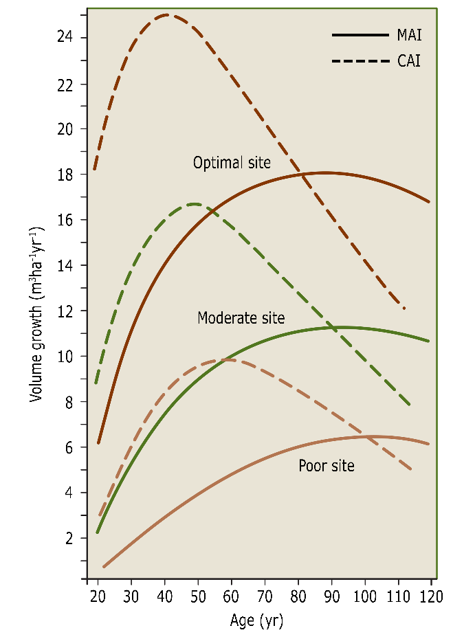
Figure 14-11: The course of current and mean annual increment at good, moderate and poor growth sites over time. The culmination point for current and mean annual increment shifts towards higher ages with lower site quality. After Assmann & Franz (1963).
Theoretically, the age at which mean annual increment culminates in an even-aged stand, indicates the optimal rotation length to obtain the highest possible stem volume or biomass production for a given tree species at a given site. The use of this production indicator only, leads to relatively short rotations. This would typically yield raw materials for low quality applications such as firewood or fibre wood (for paper or fibre board applications). When larger dimensions and higher wood quality are desired, rotation length has to be increased. Stems develop knot-free logs with a sufficiently thick layer of knot-free wood for use for veneer or furniture only at higher ages. Large dimension sawn timber also requires larger stem dimensions, with higher prices per unit volume for older and larger stems. Thus despite lower average growth over a longer rotation period, higher financial yield can be achieved. This means that the culmination of the value gain (in € yr-1 for a tree or in € ha-1yr-1 for a stand) usually occurs at a later age (fig. 14-12), provided that the average stem quality allows high-end applications. Also, stand regeneration by natural seeding requires longer rotation periods to allow for sufficient seed production.
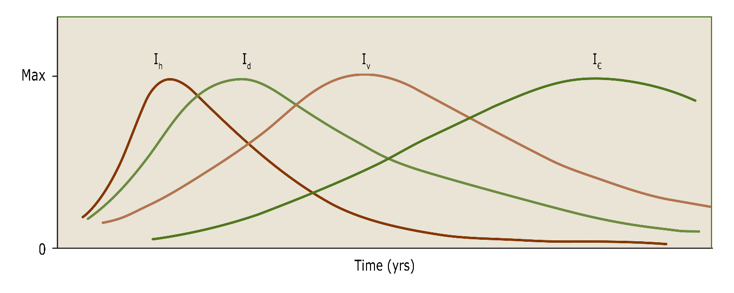
Figure 14-12: Generalized curves of the annual increment of height (Ih), diameter (Id), volume (Iv) and value per m3 (I€) of a tree. The culmination of increment falls at different times for the different variables.
When calculating the volume of trees and stands, and for determining their increment, the basal area is used. Basal area is defined as the cross-sectional area of a single stem (tree basal area), or summed over all stems in a stand (stand basal area), at breast height. For an individual tree, it can be derived directly from the measured diameter (DBH) using:
![]()
When not dbh but circumference (c) is measured, the basal area is equal to:
![]()
The stand basal area is the sum of all individual tree basal areas per hectare, expressed in m2 ha-1. This is a common measure of stand density, as it combines tree density and tree size. Stand basal area tends to reach a maximum value in dense stands. Many thinning guidelines are based on optimal basal area development over time, based on experimental plots. For shade-tolerant tree species, a higher basal area can be maintained compared to light-demanding species.
Various measurement protocols have been developed to determine the volume of a stand (see classical text books such as Kershaw et al. 2016). Essentially, the volume of a tree can be estimated by multiplying the basal area with height, and correcting for tree taper using a tree form factor to compensate for the difference between a cylinder and the actual tree shape (see Box 14-2 on tree shape and stand volume).
The volume of a stand can be estimated by multiplying stand basal area with a measure of stand height, usually the dominant height, and correcting for general tree shape using an stand form factor reflecting the average taper of the trees. The tree form factor in general lies between 0.3 and 0.5, reflecting a general stem shape between a cone (form factor = 0.33) and a paraboloid (form factor = 0.5).
The average height of the stand can be approximated by taking the height of the tree with the quadratic mean diameter (dq), i.e. the tree with the average basal area in the stand (Table 14-1). Although this quadratic mean height (hq) is slightly larger than the actual average height, it can be used to estimate the volume of the stand (Prodan 1965). If the volume of the tree with quadratic mean diameter (vq) is known, stand volume (V in m3 ha-1) can be estimated by multiplying the volume of the tree with mean quadratic diameter by the stem number (N) using V ≈ N ∙ vq .
A more accurate, but also more intensive, method to estimate stand volume is to do measurements on the actual tree population, based on circular sample plots, or a complete tally of diameters and heights of all trees. The literature on methods of forest inventory and wood geometry is large. For more detailed considerations, see overview books such as Philip (1994), Van Laar & Akça (2007), Kershaw et al. 2017 and West (2009). For more details on forest inventories, see chapter 33).
Root growth and longevity widely differ across different root categories, notably coarse roots, transport fine roots and absorptive fine roots (see chapter 12.5). The growth and resulting architecture of the coarse-root system generally depends on environmental conditions and is species- or genus-specific (see chapter 12.7.4). Coarse root turnover is infrequent and occurs in association with strong disturbances and/or tree mortality.
Root growth rates and lifespan are not commonly distinguished between transport and absorptive fine roots, but the lifespan of absorptive first- to third-order roots must be overall lower than that of their higher-order parent roots. Generally, fine roots that remain non-woody throughout their life (so-called ‘short roots’, fibrous roots’ or ‘brachyrhiza’) have a lifespan of about one year in temperate tree species, but this value was found to vary between 8 months and 2.5 years across temperate tree species (Withington et al. 2006). They grow in length rather than diameter, so they do not exhibit secondary growth, and elongation rates are dependent on root morphology – for example, thin absorptive roots generally grow faster than thick absorptive roots. Their growth through the soil substrate is facilitated by the root cap or calyptra (fig. 12.24), a protective layer around the root tips that secretes a slimy substance to minimize root damage. The root cap contains starch granules (amyloplasts) that shift to the bottom of a cell due to gravity, providing the plant with a sense direction and causing the roots to grow downwards (gravitropism). From the meristem at the root tip, new root cap cells are continuously formed downwards.
A small part of the first-order roots develop into ‘long roots’ (also: ‘pioneer roots’ or ‘macrorhiza’). They exhibit secondary growth and develop into highly branched, higher order, woody roots that form the physical framework of the root system from which lower order roots grow. These different root types also differ in their growth rates, e.g., pioneer roots of Quercus rubra were found to grow 5 – 10 mm per day, whereas the distal, non-woody roots elongated at a rate of 2 mm per day (Lyford 1980). The (diameter) growth of coarse roots generally follows the same principles as that of the stem.
Both growth and mortality of fine roots are contingent on environmental conditions, such as (soil) temperature and moisture availability. Tree root growth often ceases below 4 – 6 °C. Root mortality increases during long dry periods and new roots will form again when soil moisture is replenished. Generally, in environments where water and/or nutrients, rather than light, constrain tree growth, trees allocate more resources to produce root biomass in order to acquire limiting soil resources. Within an individual root system, root growth and biomass often increase in places with high soil resource availability. For example, because soil nutrients and (rain) water are often most abundant in the top soil (where nutrients become available through litter decomposition and mineralization), the majority of absorptive tree roots are generally located in the top 20 cm of the soil, and do not exceed 1 m soil depth in temperate forests. Here, to exploit the soil volume, up to thousands of km of fine roots can be present in the soil per hectare (Table 14-3). The total root volume typically remains considerably less than the volume of the above-ground parts (Table 14-3), with root/shoot volume ratios of about 1:5 in temperate climate zones, although this ratio may thus vary depending on above- versus belowground resource limitations and concomitant responses in biomass allocation.
The timing of root growth is typically asynchronous to shoot growth. In response to hormonal signals the growth of roots generally starts well before that of aboveground plant parts to supply the shoots with water and nutrients needed for bud flush (but these patterns may differ between tree species, fig. 14-13). Root growth may also be terminated later in the growing season than aboveground growth owing to the buffered climate of the soil where temperatures decrease more gradually than air temperatures, so that roots may experience a longer growing season than shoots.
Table 14-3: Root characteristics (per ha) of three types of forest stands on a moraine soil in Denmark. Source: Holstener-Jørgensen (1958).
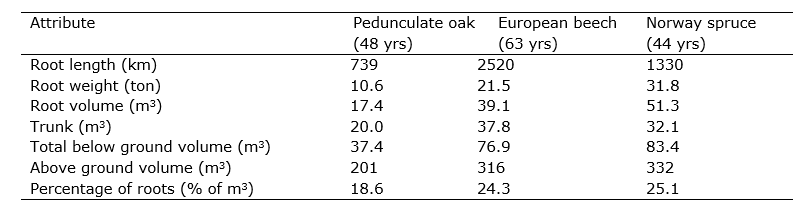
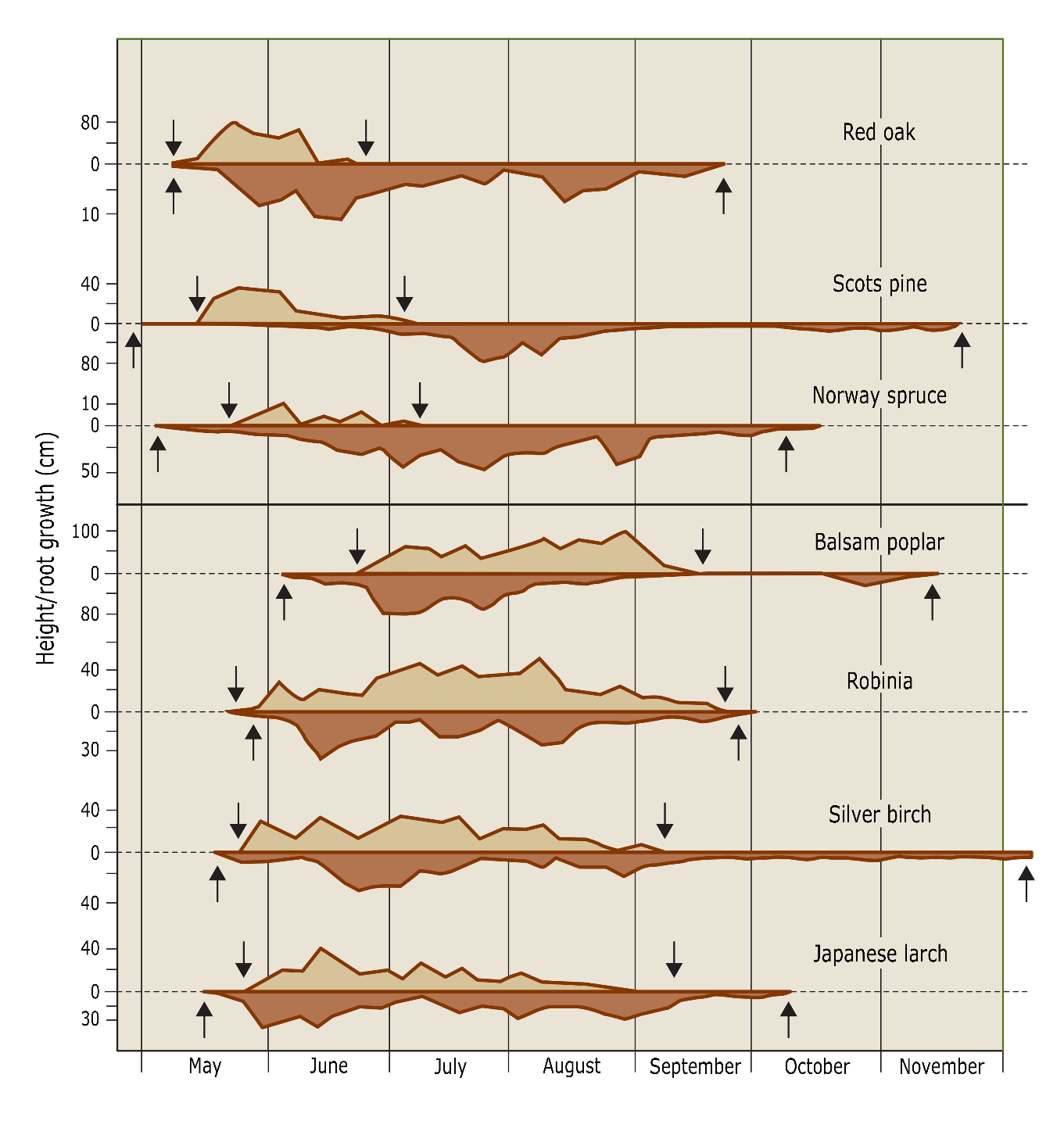
Figure 14-13: Variation in the elongation of the top shoot (above zero line) and of the roots (below zero line) during the growing season for seven tree species in Eberswalde (D). The arrows indicate the beginning and end of the growth period. (Lyr et al. 1992).
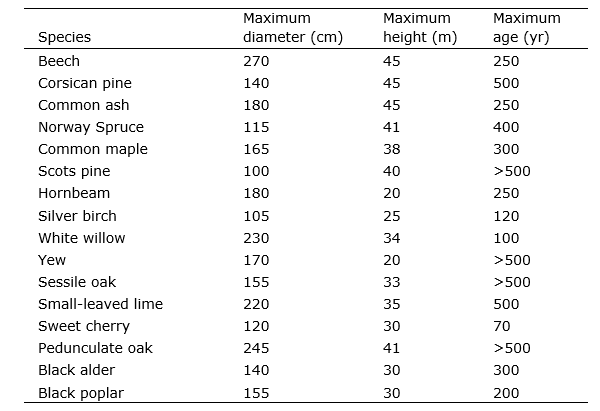
Based on the rhythm of height and diameter growth, the life cycle of a tree can be divided into three stages: the juvenile phase dominated by height growth, the adult phase dominated by diameter growth, flowering and seed production, and the senescent phase characterized by decrease in crown density and eventually deterioration of the entire crown (fig. 14-14). The rate at which these phases succeed each other is species-specific and determines the preferred harvest age. Note that pioneer tree species with high light demands tend to have a short life span, while shade-tolerant late-successional species may reach much higher ages. Birch, willow, poplar and cherry trees have a relatively short life span not exceeding more than 100-150 years. Oak and lime on the other hand, may reach ages of several hundreds of years (Table 14-4).
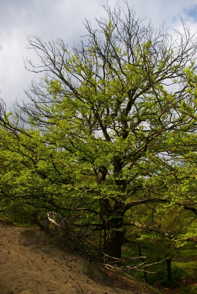
Figure 14-14: Declining beech on a sand dune (Veluwe area, Netherlands). During the senescent phase, the crown slowly degenerates and the leaves concentrate more and more around the crown base. Photo Jan den Ouden.
Table 14-4: Maximum diameter, height and age of some important tree species in European forests. Data collected by L. Goudzwaard.
Trees vary in growth rate, depending on their age, their genetic predisposition and the availability of growth factors such as light, water and nutrients. In the end, very large differences may arise in final tree size. For example, on very dry and acidic soils, Scots pines do not grow much taller than 10-15 m, while on a rich soil with good moisture supply, the same species may easily reach 30 m in height. In the deep shade, a beech may not have grown much taller than a few meters over a period of a 100 years, while in full light, in the same time and at the same site, a beech tree may grow up to a height of over 40 meters.
The large variation in independent site factors for tree growth, such as climate and soil conditions, is clearly reflected in the differences in site productivity for a given tree species observed between stands, forests or regions (Table 14-5). Furthermore, tree species may have an effect on soil formation and soil organic matter, via their litter quality (see chapter 21) and hence may influence water availability and nutrient supply of the soil (Hommel et al. 2007). This also strongly influences the growth of trees, and the herbaceous flora under the canopy, and depending on the tree species, large differences in growth and tree vitality may occur on a small spatial scale.
This section first discusses the relationship between the growth of individual trees and the growth of a stand. Growth differences between stands are discussed based on expected growth in relation to site quality. At the end, models to predict tree and stand growth are briefly introduced.
14.7.1 From tree increment to stand growth
For many reasons, e.g. to determine the influence of different soil types on growth, it is important to translate individual tree increment into the growth of an entire stand. Usually, it is not possible to accurately monitor the specific growing conditions of an individual tree in a stand, e.g. because the exact location of the roots cannot be determined in a non-destructive way. Also, light interception by individual crowns cannot be determined with simple measurements. At the stand level, however, it is possible to determine the total amount of available radiation, or the moisture availability in the rooted profile. Thus, when assessing growth in relation to site factors, the total growth per unit of area (per hectare) is a more suitable variable to consider.
The diameter growth of individual trees is not a good indicator of site quality. When stem number is high, diameter increment per tree will be lower at a certain stand growth level as compared to a stand with lower stem number. Basal area increment (in m2 ha-1 yr-1) is therefore a more appropriate measure to describe growth of a stand.
14.7.2 Yield class and increment prognosis
Given the long life span of trees, the prediction of growth in forestry is important. In the past, much attention has been paid to the development of empirical yield tables to describe growth (Table 14-6). These are empirical models describing the development of stand volume, basal area, tree height and other stand characteristics over the entire life time (rotation period) of a given tree species, usually in even-aged monocultures, and separated by site class. Such tables are based on empirical data from permanent forest plots, and apply to stands of a particular tree species with the same thinning regime in a specific geographical region. Yield tables can be used for a quick assessment of increment, and for the prediction of yields from thinning and final felling. They also serve as a standard or guideline for thinning treatments.
The growth potential of a tree species for a specific site is called yield class or site class. The yield class can be expressed directly as the maximum average annual volume increment (in m3 ha-1 yr-1), or categorized as yield or site classes (Table 14-6, Fig. 14-15). Volume growth is strongly correlated with height growth. This is reflected in Eichhorn’s law (1904), which states that at a certain average stand height, the volume is the same regardless of the site quality of the stand. In later studies, it became clear that this was not valid under all conditions (Prodan 1965), but it clearly indicates that stand height (at a certain age) provides a good measure for estimating stand volume and productivity. The yield classes in the yield tables are therefore often defined on the basis of dominant height, attained at a certain age (Fig. 14-15).
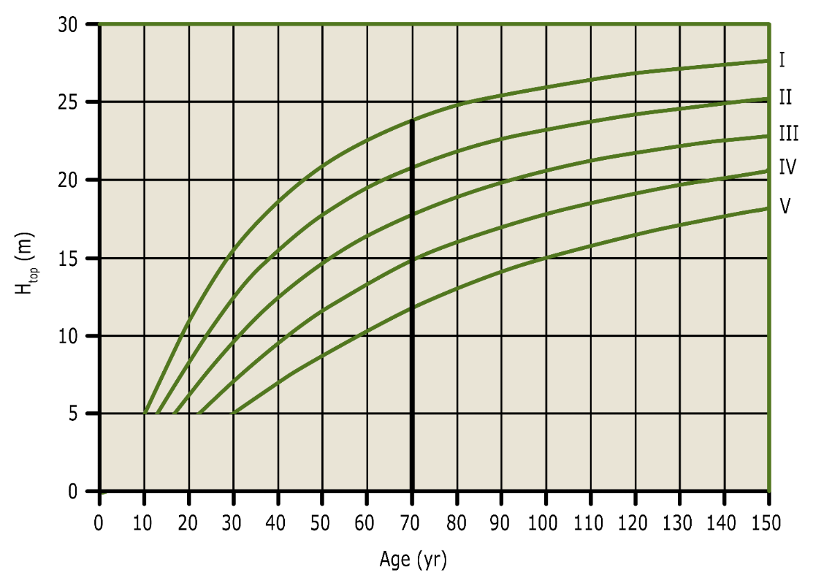
Figure 14-15: Height curves of Scots pine for different site classes in the Dutch yield table for Scots pine (Jansen et al. 2018). The relative site classes are classified by height growth (top height at age = 70 yr). By determining the top height of a stand at a given age, the site class can be inferred from the graph.
Table 14-5: Relationship between site class, dominant height and volume production for beech in Belgium. Here, Hdom is the dominant tree height at age 100 yr; Im is the mean annual increment over 100 yr.
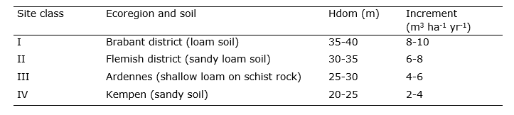
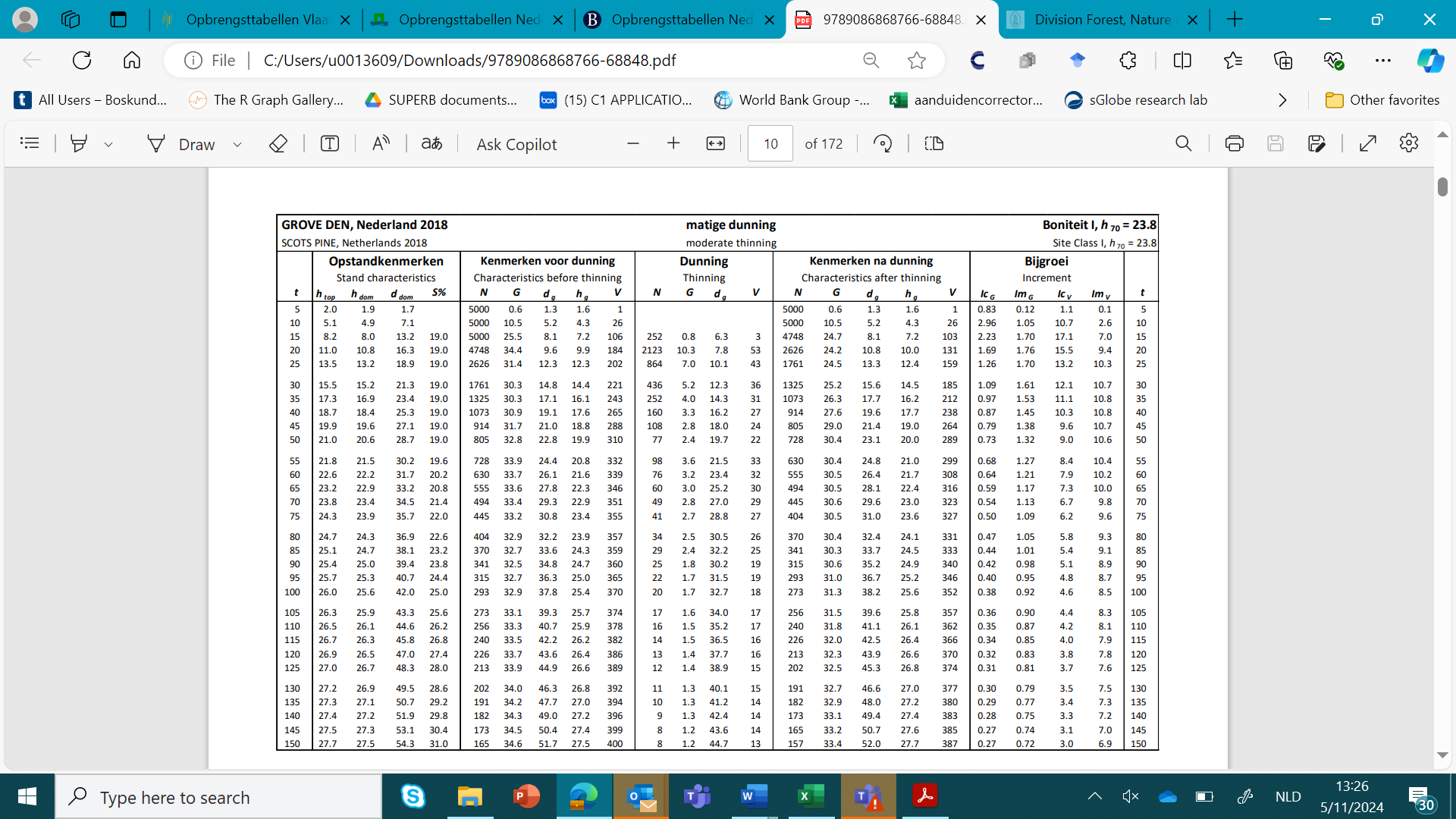
Table 14-6: Example of a yield table for Scots pine managed with moderate thinning and located on site class I, which corresponds to a dominant height at age 70 years (h70) of 23.8m (from Jansen et al., 2018, see also Fig. 14-15), with t = age (yr), htop = top height (m), hdom = dominant height (m), ddom = mean diameter of dominant tree, S% = Hart-Becking spacing index, N = stand density (ha-1), G = stand basal area (m2 ha-1), dg = quadratic mean diameter (cm); hg = mean height of tree with dg (m); V = stand volume over bark (m3 ha-1), IcG = current annual basal area increment at age t (m2 ha-1yr-1), ImG = mean annual basal area increment (m2 ha-1yr-1), IcV = current annual volume increment at age t (m3 ha-1 yr-1), ImV = mean annual volume increment (m3 ha-1 yr-1).
In the development of yield tables, and also in other studies that model tree growth, generalized functions are used to describe the development of particular tree characteristics over time, based on measurements on permanent field plots, usually in even-aged stands. Increment curves can be of various mathematical forms, depending on the purpose and on data availability. Increment curves are derived by fitting the most appropriate mathematical formula to empirical tree growth data. One of the most commonly used expressions for estimating growth of homogeneous even-aged stands in relation to site quality is the so-called Chapman-Richards equation:
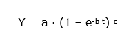
with Y = the variable to be predicted, a = a maximum value that variable Y may reach (asymptote), b = parameter describing the growth rate, and c = a shape parameter for the expression and t = age of the tree or stand. The Chapman-Richards function has been widely used for modelling height growth, as height tends to reach a maximum at higher stand age (the asymptote a in the expression). The increase of basal area with age can also be described with the Chapman-Richards function.
An important limitation of the empirical yield tables is that they do not take into account any changes in growing conditions during the life of a stand. For example, Spiecker et al. (1996) have shown that the majority of older stands in Europe have increased in productivity during their life span, comparable to at least one site class, as a result of nitrogen and CO2 fertilization (Pretzsch et al 2024; Etzold et al 2020). Furthermore, yield tables are limited to the stand and site conditions of the field plots on which they are based. For example, the German or Dutch growth tables are not suitable for the beech stands in the Sonian Forest in Belgium. These beech stands show a significantly slower growth in their youth (during the first 40 years) due to the presence of a strongly compacted and decalcified upper soil layer. At a later age (from 120 years) these stands exhibit a stand increment that is higher than the best site class from the yield tables mentioned, after the root systems have extended into calcareous loess layers at a depth of more that 3m (see De Vos, 2005).
In contrast to empirical growth models such as yield tables, mechanistic growth models explicitly take into account the influence of individual growth factors, making it possible to predict growth under changing conditions. Mechanistic models are based on the ecological and physiological processes underlying growth (photosynthesis, respiration, evapotranspiration, etc.) and may simulate the growth of a stand based on ecological processes (e.g. Storms et al. 2025). The disadvantage of these models is their high degree of complexity and high data requirement on site conditions and species-specific parameters characterizing physiological processes. Combined with the uncertainties in the quantification of the most important physiological processes, this means that mechanistic models are particularly suitable for research on forest ecosystems – particularly for testing hypotheses through simulation experiments- and less suitable for growth prediction in a concrete situation. Promising alleys to predict forest growth under climate change are hybrid models, which combine the predictive capacity of mechanistic models with the accuracy of empirical models (e.g. Storms et al. 2022).
In yield tables, a volume function based on a regression equation is often used, calibrated on section measurements of a sufficiently large number of felled logs. A commonly used volume function is v = a × DBH b× L c, which is a more general form of the expression : v = f × p × (DBH/200)2 × L. This relationship between DBH, h and v is then given in so-called volume tables. For a specific forest inventory, a relationship between the diameter and the tree volume can first be derived by measuring a number of sample trees in an area and applying the volume table. By regression analysis, a relationship can then be established between DBH and v, usually using a second-degree polynomial. The resulting volume table then takes the form: v = a + b × DBH + c × DBH2.
Assmann (1961), Mitscherlich (1978), Lyr et al. (1992), Pretzsch (2009).
Assmann, E. 1961. Forest yield science. FSVO, Munich.
Assmann, E. & F. Franz 1963. Preliminary spruce yield table for Bavaria. Institute of Yield Science of the Forstliche Forschungsanstalt München, Munich.
Balleux, P. & Q. Ponette 2006. Spruce thinning device, principles lessons from thirty years of experience. Walloon Forest 83: 3-21.
Berman, M. E. & T. M. De Jong. 1997. Diurnal patterns of stem extension growth in peach (Prunus persica): Temperature and fluctuations in water status determine growth rate. Physiologia Plantarum 100: 361-370.
Dagnelie, P., Palm, R., Rondeux, J., Thill, A., 1988. Production tables relating to common spice. Les Presses agronomiques de Gembloux.
Deckmyn, G., H. Verbeeck, M. Op de Beeck, D. Vansteenkiste, K. Steppe & R. Ceulemans 2008. ANAFORE: a stand-scale process-based forest model that includes wood tissue development and labile carbon storage in trees. Ecological Modeling 215: 345–368.
De Vos, B., 2005. Soil compaction and the influence on the natural rejuvenation of Beech in the Sonian Forest. Institute for Forestry and Wildlife Management, Report IBW Bb 2005.004.
Eichhorn, F. 1904. Relationships between stock level and inventory mass. Allgemeine Forst und Jagdzeitung 80: 45–49.
Etzold, S., Sterck, F., Bose, A.K., Braun, S., Buchmann, N., Eugster, W., Gessler, A., Kahmen, A., Peters, R.L., Vitasse, Y. and Walthert, L., 2022. Number of growth days and not length of the growth period determines radial stem growth of temperate trees. Ecology Letters, 25(2), pp.427-439.
Holstener-Jørgensen, H. 1958. Investigation on root systems of oak, beech, and Norway spruce on groundwater affected moraine soils with a contribution to elucidation of evapotranspiration of stands. Forstlige Forsögsväsen I Danmark, Bd. 25, 225–290.
Houtzagers, M.R. & P. Schmidt 1994. The reaction of poplar clones to competition in relation to growth space. Hinkeloord Reports 12, Wageningen Agricultural University.
Jager, K. & A. Oosterbaan 1994. Construction of mixed hardwood plantings with native species. Schuyt & Co, Haarlem, The Netherlands.
Jansen, H. (Ed.), Oosterbaan, A. (Ed.), Mohren, G. M. J., Goudzwaard, L., den Ouden, J., Schoonderwoerd, H., Thomassen, E. A. H., Schmidt, P., & Copini, P. (2018). Opbrengsttabellen Nederland 2018. Wageningen Academic Publishers. https://doi.org/10.3920/978-90-8686-876-6.
Kershaw Jr, J.A., Ducey, M.J., Beers, T.W. and Husch, B., 2017. Forest mensuration. John Wiley & Sons.
Leibundgut, H, S. Dafis & F. Richard 1963. Studies on root growth of different tree species. Schweizerische Zeitschrift für Forstwesen 114: 621-646.
Lyford, W. H., 1980. Development of the root system of northern red oak (Quercus rubra L.). Harvard University, Harvard Forest. Cambridge, MA, USA.
Lyr, H., H.J. Fiedler & W. Tranquilini 1992. Physiologie und Ökologie der Gehölze. Gustav Fisher Verlag, Jena.
Mitscherlich, G. 1978. Wald, Wachstum und Umwelt. Volume I: Form and Growth of Baumund Bestand. Frankfurt a.M., J.D. Sauerländers Verlag.
Philip, M.S. 1994. Measuring Trees and Forests. Wallingford, CABI Publishing, 2nd edition.
Pretzsch, H. 2009. Forest Dynamics, Growth and Yield. Berlin, Springer Verlag.
Pretzsch et al. 2014. Forest stand growth dynamics in Central Europe have accelerated since 1870. Nature Communications 5(1), 4967.
Etzold, S., Ferretti, M., Reinds, G. J., Solberg, S., Gessler, A., Waldner, P., … & de Vries, W. 2020. Nitrogen deposition is the most important environmental driver of growth of pure, even-aged and managed European Forests. Forest Ecology and Management 458, 117762.
Savill, P.S. & A.J. Sandels 1983 The influence of early respacing on the wood density of Sitka spruce. Forestry 56: 109-120.
Spiecker, H. K. Mielikäinen, M. Köhl, J.P. Skovsgaard (eds.) 1996. Growth Trends in European Forests. Studies from 12 Countries. European Forest Institute Research Report No. 5, Springer Verlag, Berlin.
Stiell, W.M. 1966. Red pine crown development in relation to spacing. Department of Forestry Publication 1145, Ottawa.
Storms, I., Thom, D., Verbist, B., Van Meerbeek, K., Gobin, A., Van Winckel, S., Van Orshoven, J. and Muys, B., 2025. Atlantic lowland forests face shifts in composition and structure under climatic change. Regional Environmental Change, 25(2), pp.1-16.
Storms, I., Verdonck, S., Verbist, B., Willems, P., De Geest, P., Gutsch, M., Cools, N., De Vos, B., Mahnken, M., Lopez, J. and Van Orshoven, J., 2022. Quantifying climate change effects on future forest biomass availability using yield tables improved by mechanistic scaling. Science of the total environment, 833: 155-189.
Verdonck, S., Geussens, A., Zweifel, R., Thomaes, A., Van Meerbeek, K. and Muys, B., 2025. Mitigating drought stress in European beech and pedunculate oak: The role of competition reduction. Forest Ecosystems, p.100303.
Van Laar, A. & A. Akça 2007. Forest Mensuration. Springer, Dordrecht, the Netherlands.
West, P.W. 2009. Tree and Forest Measurement. Springer Verlag, 2nd edition, Berlin.
Withington, J.M., P.B. Reich, J. Oleksyn & D.M. Eissenstat, 2006. Comparisons of structure and life span in roots and leaves among temperate trees. Ecological Monographs, 76: 381–397.
Acknowledgements
This Chapter is published on the EUROSILVICS platform, established as part of the EUROSILVICS Erasmus+ grant agreement No. 2022-1-NL01-KA220-HED-000086765.
Author affiliations:
| Bart Muys | Division of Forest, Nature & Landscape, Department of Earth & Environmental Sciences, KU Leuven, Celestijnenlaan 200E box 2411, 3001 Leuven, Belgium |
| Jan den Ouden | Forest Ecology and Forest Management Group, Wageningen University and Research, Droevendaalsesteeg 3A, 6708 PB Wageningen, Netherlands |
| Kris Verheyen | Forest & Nature Lab, Ghent University, Geraardsbergsesteenweg 267, 9090 Melle-Gontrode, Belgium |
| Monique Weemstra | Forest Ecology and Forest Management Group, Wageningen University and Research, Droevendaalsesteeg 3A, 6708 PB Wageningen, Netherlands |
| Frits Mohren | Forest Ecology and Forest Management Group, Wageningen University and Research, Droevendaalsesteeg 3A, 6708 PB Wageningen, Netherlands |