
Chapter 4: Concepts of time and scale – Download PDF
Authors: Hubert Hasenauer
Author affiliations are given at the end of the chapter
Intended learning level: Basic / Advanced / Applied (Professional)
This material is published under Creative Commons license CC BY-NC-SA 4.0.
| Purpose of the chapter: |
|---|
| Forestry decisions unfold across spatial and temporal scales. Stands change over decades through competition, disturbance and management interventions, while landscapes change over centuries with climate and policy. Attention to scale prevents mismatches, such as judging long processes based on short monitoring windows. It should guide sampling, models and the timing of silvicultural methods, such as thinning and the choice of rotation length, to align ecological dynamics with social or economic objectives. |
NOTE: this part is a full draft, which in due time will be further revised
and edited following review by the EUROSILVICS Project Board
04: Concepts of time and scale in forestry 1
4.2 Scale in silviculture and forest management 2
4.2.1 Silvicultural systems as spatio-temporal programs 2
4.2.2 Scaling pitfalls from research and practice 3
4.2.3.1 Temporal sampling, aliasing, and timing of observations. 4
4.2.3.2 Temporal scaling and “false chronosequences” 5
4.2.4 Uneven-aged systems and time and scale 5
Forestry decisions succeed or fail depending on how well they match the rhythms of time and the patterns of space. Natural processes move along at different speeds and timeframes, from photosynthesis that shifts within minutes and hours to cambial growth and phenology that unfold over seasons. Disturbances can be sudden, like gusts of wind that throw entire stands in minutes, yet their legacies persist for decades. Other processes build gradually, such as drought episodes that accumulate over weeks or months and then may impact physiology, mortality, and regeneration for years.
Spatial patterns are similarly decisive. What is visible at the tree level differs from what becomes clear at the stand or landscape level. Tree-level measurements capture competition, microclimate, and physiological response. Stands reveal structure, gap formation, and regeneration niches. Landscape views expose connectivity, disturbance regimes, and invasion fronts. The perspective through which the forest is seen can change everything, allowing us to see certain dynamics and miss others.
In forestry, scale is the spatial and temporal resolution and extent at which we observe, model, or make decisions. Grain refers to the smallest unit in space or time, such as a single tree, meter, hour, or day. Extent is the full area or period under consideration, such as a stand, landscape, decade, or century. The choice of scale has profound impacts, since many forest processes operate at scales that differ from the scales of management and policy.
Another important concept is emergence. Emergent properties arise from interactions among components and cannot be obtained by simply summing or averaging the parts. The concept of emergence may be explained through a rope (Seidl et al., 2013): Mass increases from adding fibers to rope, while stiffness and cohesion depend on how fibers interact. Transferred to forests, standing volume is additive, just like fibers in a rope. Wind resistance, resilience, and community assembly depend on the spatial arrangement, structural diversity, species composition and the way gaps form and close.
Management sits at the intersection of these ideas. Silvicultural choices such as thinning intensity, regeneration method, or species composition are made at stand scales and on decadal horizons, yet they rest on seasonal physiology and on disturbance regimes that operate across landscapes and over long periods. At a landscape level, policy instruments are designed over administrative areas and election cycles, but changes to the landscape itself emerge from many local management actions and ecological interactions. Without explicit links across scales, any plans inherit blind spots and unanticipated trade-offs.
4.2 Scale in silviculture and forest management
4.2.1 Silvicultural systems as spatio-temporal programs
Silvicultural systems are management programs that specify what happens, where it happens, and when it happens. They bundle regeneration, tending, and harvesting into a sequence that runs over a defined area and time horizon. Because they combine a schedule with a spatial layout, they encode time and space together and are the most visible place where scaling choices enter everyday forestry.
Classic silviculture is based around a particular pairing of scales: The stand became the operational spatial unit and the rotation became the dominant temporal unit. The historical root of this is the Normalwald (“normal forest”) model of Hundeshagen (1826), which pictured forests as mosaics of homogeneous, fully stocked stands delivering steady yields on fixed rotations (Hundeshagen, 1826). This vision pushed practitioners toward uniformity in composition, structure, and timing of interventions. To secure steady yields, foresters reduced stochasticity with even-aged forestry and widespread use of artificial regeneration. Outcomes became more predictable, but spatial patterns and temporal dynamics were simplified relative to natural systems, with silvicultural measures being prescribed at specified intervals.
In even-aged systems such as clearcut, seed-tree, or shelterwood forestry, the “life phases” are separated in time. Stand establishment is followed by a period of tending and then by a regeneration harvest at maturity. The sequence sets a rotation or cutting cycle that combines thinning intensity and timing. The spatial unit is the stand, treated as uniform enough in composition, age distribution, and site quality to justify a single prescription across the whole area.
4.2.2 Scaling pitfalls from research and practice
A large share of the classic evidence base in forestry came from small, highly homogeneous research plots, yet the results were then applied to much larger, more heterogeneous stands. Small plots were attractive for scientists: they are easier to keep uniform, allow many replications, and are cheaper to measure. The widespread use of scale-independent units like trees per hectare further encouraged the idea that averages across a plot would scale linearly to stands. In reality, this relies on the assumptions of linearity and homogeneity that often fail under operational conditions (Puettmann et al., 2009).
These problems show up most clearly when disturbances and operational side effects are no longer controlled. In practice, yields and growth responses are frequently lower than trial expectations because unmodeled factors such as harvest damage, thinning shock, windthrow, diseases and pests or drought reduce stand performance. Once disturbances are treated as a part of forest development rather than external anomalies, the systematic over-prediction of growth and yield by traditional tools becomes understandable.
Regeneration dynamics highlight the same scaling trap. Key ecological mechanisms function at different spatial grains: seed availability depends on parent-tree proximity and stand structure ranging from meters to hundreds of meters, while seedbed quality varies at the microsite but is shaped by local canopy conditions. Designs that average the stand can therefore miss the mixed scales that actually control establishment of regeneration following a harvest.
Large, operational-scale experiments were created to confront these issues. They used treatment units on the order of entire blocks and combined structural retention with openings to study responses across microsite, gap, and treatment-unit scales. It becomes obvious that many silvicultural questions are not best answered at the treatment-unit (stand-average) scale. They require sampling and analysis at the scale of mechanism (gaps, light gradients, neighborhoods), rather than averaging them.
4.2.3.1 Temporal sampling, aliasing, and timing of observations.
Time scale is not just about how long processes take; it is also about how often and when we observe them. If the sampling interval is less fine than the process of interest, aliasing turns fast pulses into noise or spurious trends. For example, drought periods lasting weeks that drive later mortality vanish inside annual summaries, and shifting measurement dates within the growing season can look like a change in growth rather than a change in timing.
Tree-ring analyses add a clear illustration of this constraint. They resolve growth at annual steps only, so a narrow ring cannot tell whether stress came from one severe drought or several shorter events within the same year. In other words, sub-annual forcing is aliased into a single yearly increment, and any shift in the timing of stress (for example an earlier summer drought) will be invisible unless it is accompanied by higher-frequency observations, such as precipitation data from a nearby weather station.
In forestry this issue is acute, because inventories are often annual or multi-annual while key drivers such as phenology, water stress, and disturbance events operate on days to weeks. Two practical rules follow from the scaling literature: (i) match sampling frequency to the dominant tempo of the question and report the temporal support of each metric (the window over which it averages), and (ii) be explicit when downscaling or aggregating, since inferring hourly or seasonal behavior from daily or annual data imports assumptions that can bias results if seasonal phase shifts occur (Eastaugh et al., 2013; Seidl et al., 2013). An overview of different forest-related processes in time and spaces is available in figure 4-1.
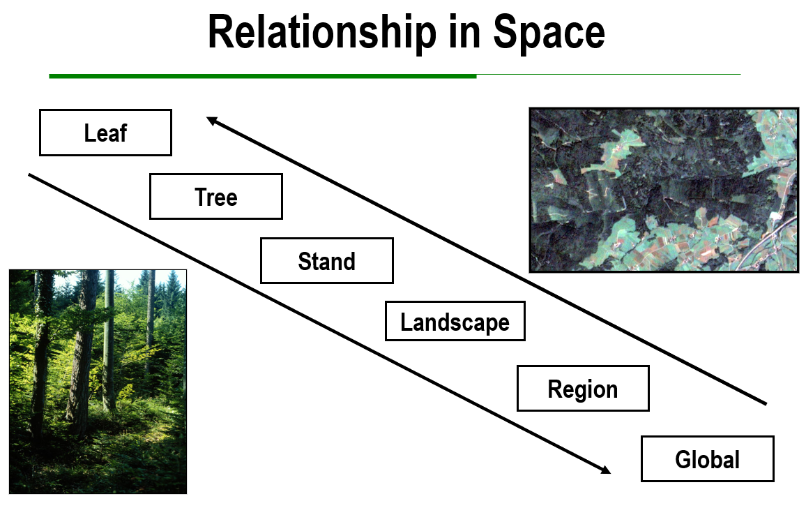
Figure 04-1: Examples of different scales in forestry.

Figure 04-2: Examples of processes across different time scales in forestry.
4.2.3.2 Temporal scaling and “false chronosequences”
Forestry is hindered by another complication: long production horizons but short observation windows. To fill gaps, we often stitch together space-for-time substitutions—different stands or cohort stages lined up and „assembled“ as if they were one time series. Without proper understanding of the underlying ecological processes, such reconstructions can create false continuity. Nonlinear processes also mean that temporal averaging can bias estimates. The safer practice is to pair any substitution with evidence on history and mechanism, and to validate at the temporal resolution relevant to decisions.
4.2.4 Uneven-aged systems and time and scale
Uneven-aged forestry reorganizes regeneration, tending, and harvesting so that these phases occur together in the same stand at any given time. Instead of creating a single cohort that is then carried to a regeneration harvest, managers maintain a reverse-J diameter distribution with continuous recruitment of small trees, growth into larger size classes, and periodic removals. The spatial grain is rather fine.
Interventions are then applied to single trees or small groups, and regeneration occurs beneath a partially retained canopy. Cutting cycles define the temporal rhythm, often between five and twenty years, but state variables such as q-ratios and target diameter distributions are the real control mechanisms.
Because multiple phases are occuring in the same space, the relevant processes live at neighborhood and microsite scales. Seedfall depends on the identity and spacing of the mother trees. Light and moisture regimes vary sharply over a few metres due to crowns, small gaps, and topographic breaks (microrelief). Soil disturbance from skidding or cable corridors can both create and destroy suitable seedbeds in a pattern that is highly localized. As a result, the success of regeneration and recruitment hinges more on the mosaic of gap sizes, edge exposure, and local competition than on stand-mean values.
Uneven-aged systems redistribute growth rather than trying to maximize it in a single cohort. Removing selected competitors frees growing space for the best-formed residuals, and repeated light entries can keep crowns deep and vigorous. In shade-tolerant or mid-tolerant mixtures this can sustain high quality timber while maintaining cover, deadwood development, and microclimate suitable for many forest interior species. At the stand level, disturbance is spread out in space and time, which can reduce variance in yields and reduce some risks associated with a single regeneration harvest.
There are limits and risks that follow directly from scale. Recruitment under a more or less permanent canopy is inherently variable through time, especially for species that require pulses of light or specific seedbed conditions. If the spatial pattern of harvesting does not periodically create gaps of the right size, regeneration can stall and the stand can gradually shift toward the most shade-tolerant species. Conversely, if gaps are repeatedly too large, regeneration can be dominated by opportunistic species and browsing pressure can concentrate along edges. True selection cutting must be distinguished from target diameter cutting. The former regulates both structure and composition using targets for basal area and size-class distribution, while the latter removes the largest trees without securing recruitment and will often degrade structure and value over time.
Operationally, repeated entries increase exposure to cumulative soil disturbance and damage to residual stems if harvesting is not carefully managed. Planning therefore benefits from a semi-permanent network of extraction trails, explicit limits on trafficked area, and retention rules that identify seed trees, habitat trees, and structural legacies. Monitoring should track not only stand totals but also the distribution of light, regeneration density by microsite, browsing intensity, and the progression of tagged cohorts through size classes. These indicators reveal whether the stand is actually following the intended diameter distribution or drifting toward structural simplification.
Uneven-aged forestry is a useful bridge between stand-focused operations and landscape objectives. Continuous canopy and frequent small disturbances support interior microclimates, seed dispersal across short distances, and gradual development of deadwood and vertical structure. At the same time, landscape-level aims such as connectivity, early-successional habitat, or fire management may require a mix of stand structures and some larger openings. The practical task is to place uneven-aged stands within a wider pattern so that the combined portfolio delivers both local and landscape functions.

Figure 04-3: Time and scale – Old Tjikko, a Norway spruce (Picea abies) in Fulufjället, Sweden. Genet age ~9,550 years; the current stem is young. What counts as “a tree” depends on scale.
Forests are structured across spatial and temporal scales, and many attributes only exist or make sense at particular levels. Additive quantities such as volume behave differently from emergent properties such as resilience, which depend on interactions and pattern. Observations and models are defined by grain and extent, and results change when either is altered. Through time, nonlinear responses, thresholds, and lagged effects mean that averages do not reliably represent system behavior. Annual records like tree rings integrate sub-annual variability into single values, while legacies from past disturbance or management shape present states. Cross-scale interactions link local neighborhoods to landscape dynamics and connect ecological processes to social and economic systems. Any translation across scales introduces assumptions and uncertainty. For these reasons, scale and time are not peripheral considerations but fundamental dimensions that govern what can be measured, inferred, compared, and ultimately managed in forestry.
Practical take-aways for system design considering space and time
Match the unit of intervention to the unit of process. Use cohorts and blocks when stand-scale processes dominate. Use gaps, groups, and dispersed retention when regeneration niches, competition, or habitat depend on neighborhoods and microsites. Then monitor within treatments, not just stand means.
Be explicit about disturbance and operational noise. Expect yield reductions from damage, shock, and weather risks that controlled trials suppress. Treat these as part of the baseline, not anomalies.
State your time assumptions. Rotations and cutting cycles should be weighed against ecological tempos like decadal wood-decay and late-successional habitat windows. Avoid building policy on chronosequences that ignore legacies and nonlinearity.
Eastaugh, C.S., Korjus, H., Kangur, A., Kiviste, A., 2013. Scaling Issues and Constraints in Modelling of Forest Ecosystems: a Review with Special Focus on User Needs. Balt. For. 19, 316–330.
Hundeshagen, J.C., 1826. Die Forstabschätzung auf neuen wissenschaftlichen Grundlagen, 1st ed. Laupp, Tübingen.
Puettmann, K.J., Coates, K.D., Messier, C.C., 2009. A critique of silviculture: managing for complexity. Island Press, Washington, DC.
Seidl, R., Eastaugh, C.S., Kramer, K., Maroschek, M., Reyer, C., Socha, J., Vacchiano, G., Zlatanov, T., Hasenauer, H., 2013. Scaling issues in forest ecosystem management and how to address them with models. Eur. J. For. Res. 132, 653–666. https://doi.org/10.1007/s10342-013-0725-y
This Chapter is published on the EUROSILVICS platform, established as part of the EUROSILVICS Erasmus+ grant agreement No. 2022-1-NL01-KA220-HED-000086765.
This text was based on two papers HH contributed to (Eastaugh et al., 2013 and Seidl et al., 2013).
Author affiliation:
| Hubert Hasenauer | Institute of Silviculture, University of Natural Resources and Life Sciences Vienna, Austria |